Computationally Efficient Convolved Multiple Output Gaussian Processes

Computationally Efficient Convolved Multiple Output Gaussian

Processes

Mauricio A. ´Alvarez∗ [email protected]

School of Computer Science University of Manchester Manchester, UK, M13 9PL

Neil D. Lawrence† [email protected]

School of Computer Science University of Sheffield Sheffield, S1 4DP

Editor: Carl Edward Rasmussen

Abstract

Recently there has been an increasing interest in regression methods that deal with multiple out-puts. This has been motivated partly by frameworks like multitask learning, multisensor networks or structured output data. From a Gaussian processes perspective, the problem reduces to spec-ifying an appropriate covariance function that, whilst being positive semi-definite, captures the dependencies between all the data points and across all the outputs. One approach to account for non-trivial correlations between outputs employs convolution processes. Under a latent function interpretation of the convolution transform we establish dependencies between output variables. The main drawbacks of this approach are the associated computational and storage demands. In this paper we address these issues. We present different efficient approximations for dependent out-put Gaussian processes constructed through the convolution formalism. We exploit the conditional independencies present naturally in the model. This leads to a form of the covariance similar in spirit to the so called PITC and FITC approximations for a single output. We show experimental results with synthetic and real data, in particular, we show results in school exams score prediction, pollution prediction and gene expression data.

Keywords: Gaussian processes, convolution processes, efficient approximations, multitask

learn-ing, structured outputs, multivariate processes

1. Introduction

Accounting for dependencies between model outputs has important applications in several areas. In sensor networks, for example, missing signals from failing sensors may be predicted due to correla-tions with signals acquired from other sensors (Osborne et al., 2008). In geostatistics, prediction of the concentration of heavy pollutant metals (for example, Copper), that are expensive to measure, can be done using inexpensive and oversampled variables (for example, pH) as a proxy (Goovaerts, 1997). Within the machine learning community this approach is sometimes known as multitask learning. The idea in multitask learning is that information shared between the tasks leads to

proved performance in comparison to learning the same tasks individually (Caruana, 1997; Bonilla et al., 2008).

In this paper, we consider the problem of modeling related outputs in a Gaussian process (GP). A Gaussian process specifies a prior distribution over functions. When using a GP for multiple related outputs, our purpose is to develop a prior that expresses correlation between the outputs. This information is encoded in the covariance function. The class of valid covariance functions is

the same as the class of reproducing kernels.1 Such kernel functions for single outputs are widely

studied in machine learning (see, for example, Rasmussen and Williams, 2006). More recently the community has begun to turn its attention to covariance functions for multiple outputs. One of the paradigms that has been considered (Teh et al., 2005; Osborne et al., 2008; Bonilla et al., 2008) is known in the geostatistics literature as the linear model of coregionalization (LMC) (Journel and Huijbregts, 1978; Goovaerts, 1997). In the LMC, the covariance function is expressed as the sum of Kronecker products between coregionalization matrices and a set of underlying covariance functions. The correlations across the outputs are expressed in the coregionalization matrices, while the underlying covariance functions express the correlation between different data points.

Multitask learning has also been approached from the perspective of regularization theory (Ev-geniou and Pontil, 2004; Ev(Ev-geniou et al., 2005). These multitask kernels are obtained as generaliza-tions of the regularization theory to vector-valued funcgeneraliza-tions. They can also be seen as examples of LMCs applied to linear transformations of the input space.

In the linear model of coregionalization each output can be thought of as an instantaneous mix-ing of the underlymix-ing signals/processes. An alternative approach to constructmix-ing covariance func-tions for multiple outputs employs convolution processes (CP). To obtain a CP in the single output case, the output of a given process is convolved with a smoothing kernel function. For example, a white noise process may be convolved with a smoothing kernel to obtain a covariance function (Barry and Ver Hoef, 1996; Ver Hoef and Barry, 1998). Ver Hoef and Barry (1998) and then Hig-don (2002) noted that if a single input process was convolved with different smoothing kernels to produce different outputs, then correlation between the outputs could be expressed. This idea was introduced to the machine learning audience by Boyle and Frean (2005). We can think of this approach to generating multiple output covariance functions as a non-instantaneous mixing of the base processes.

The convolution process framework is an elegant way for constructing dependent output pro-cesses. However, it comes at the price of having to consider the full covariance function of the

joint GP. ForD output dimensions and N data points the covariance matrix scales as DN

lead-ing toO(N3D3)computational complexity andO(N2D2)storage. We are interested in exploiting

the richer class of covariance structures allowed by the CP framework, but reducing the additional computational overhead they imply.

In this paper, we propose different efficient approximations for the full covariance matrix in-volved in the multiple output convolution process. We exploit the fact that, in the convolution framework, each of the outputs is conditional independent of all others if the input process is fully observed. This leads to an approximation that turns out to be strongly related to the partially in-dependent training conditional (PITC) (Qui˜nonero-Candela and Rasmussen, 2005) approximation for a single output GP. This analogy inspires us to consider a further conditional independence

assumption across data points. This leads to an approximation which shares the form of the fully in-dependent training conditional (FITC) approximation (Snelson and Ghahramani, 2006;

Qui˜nonero-Candela and Rasmussen, 2005). This reduces computational complexity toO(N DK2)and storage

toO(N DK)with K representing a user specified value for the number of inducing points in the approximation.

The rest of the paper is organized as follows. First we give a more detailed review of related work, with a particular focus on relating multiple output work in machine learning to other fields. Despite the fact that there are several other approaches to multitask learning (see for example Caru-ana, 1997, Heskes, 2000, Bakker and Heskes, 2003, Xue et al., 2007 and references therein), in this paper, we focus our attention to those that address the problem of constructing the covariance or kernel function for multiple outputs, so that it can be employed, for example, together with Gaus-sian process prediction. Then we review the convolution process approach in Section 3 and Section 4. We demonstrate how our conditional independence assumptions can be used to reduce the com-putational load of inference in Section 5. Experimental results are shown in Section 6 and finally some discussion and conclusions are presented in Section 7.

2. Related Work

In geostatistics, multiple output models are used to model the co-occurrence of minerals or pollu-tants in a spatial field. Many of the ideas for constructing covariance functions for multiple outputs have first appeared within the geostatistical literature, where they are known as linear models of coregionalization (LMC). We present the LMC and then review how several models proposed in the machine learning literature can be seen as special cases of the LMC.

2.1 The Linear Model of Coregionalization

The term linear model of coregionalization refers to models in which the outputs are expressed as

linear combinations of independent random functions. If the independent random functions are

Gaussian processes then the resulting model will also be a Gaussian process with a positive semi-definite covariance function. Consider a set ofDoutput functions{fd(x)}Dd=1where x∈ ℜp is the

input domain. In a LMC each output function,fd(x), is expressed as (Journel and Huijbregts, 1978)

fd(x) = Q X

q=1

ad,quq(x). (1)

Under the GP interpretation of the LMC, the functions{uq(x)}Q_q=1are taken (without loss of gener-ality) to be drawn from a zero-mean GP withcov[uq(x), uq′(x′)] =kq(x,x′)ifq=q′and zero

oth-erwise. Some of these base processes might have the same covariance, this iskq(x,x′) =kq′(x,x′),

but they would still be independently sampled. We can group together the base processes that share latent functions (Journel and Huijbregts, 1978; Goovaerts, 1997), allowing us to express a given output as

fd(x) = Q X

q=1

Rq

X

i=1

where the functionsui

q(x)

Rq

i=1,i= 1, . . . , Rq, represent the latent functions that share the same

covariance functionkq(x,x′). There are nowQgroups of functions, each member of a group shares

the same covariance, but is sampled independently.

In geostatistics it is common to simplify the analysis of these models by assuming that the

pro-cessesfd(x)are stationary and ergodic (Cressie, 1993). The stationarity and ergodicity conditions

are introduced so that the prediction stage can be realized through an optimal linear predictor using a single realization of the process (Cressie, 1993). Such linear predictors receive the general name of cokriging. The cross covariance between any two functionsfd(x)andfd′(x)is given in terms of

the covariance functions forui_q(x)

cov[fd(x), fd′(x′)] = Q X

q=1 Q X

q′₌₁

Rq

X

i=1

Rq

X

i′₌₁

ai_d,qai_d′′_,q′cov[ui_q(x), ui ′

q′(x′)].

Because of the independence of the latent functionsui_q(x), the above expression can be reduced to

cov[fd(x), fd′(x′)] = Q X

q=1

Rq

X

i=1

ai_d,qai_d′_,qkq(x,x′) = Q X

q=1

bq_d,d′kq(x,x

′_{), (3)}

withbq_d,d′= PRq

i=1aid,qaid′_,q.

For a numberN of input vectors, let fdbe the vector of values from the outputdevaluated at

X={xn}Nn=1. If each output has the same set of inputs the system is known as isotopic. In general,

we can allow each output to be associated with a different set of inputs, X(d)={x(d)n }Nn=1d , this is

known as heterotopic.2 For notational simplicity, we restrict ourselves to the isotopic case, but our

analysis can also be completed for heterotopic setups. The covariance matrix for fd is obtained

expressing Equation (3) as

cov[fd,fd′] = Q X

q=1

Rq

X

i=1

ai_d,qai_d′_,qKq= Q X

q=1

bq_d,d′Kq,

where Kq∈ ℜN×N has entries given by computingkq(x,x′)for all combinations from X. We now

define f to be a stacked version of the outputs so that f= [f⊤₁, . . . ,f⊤_D]⊤_{. We can now write the}

covariance matrix for the joint process over f as

Kf,f= Q X

q=1

AqA⊤q ⊗Kq= Q X

q=1

Bq⊗Kq, (4)

where the symbol⊗denotes the Kronecker product, Aq∈ ℜD×Rq has entriesaid,qand Bq=AqA⊤q ∈

ℜD×D _{has entries b}q

d,d′ and is known as the coregionalization matrix. The covariance matrix Kf,f

is positive semi-definite as long as the coregionalization matrices Bq are positive semi-definite and

kq(x,x′) is a valid covariance function. By definition, coregionalization matrices Bq fulfill the

positive semi-definiteness requirement. The covariance functions for the latent processes,kq(x,x′),

can simply be chosen from the wide variety of covariance functions (reproducing kernels) that are

used for the single output case. Examples include the squared exponential (sometimes called the Gaussian kernel or RBF kernel) and the Mat´ern class of covariance functions (see Rasmussen and Williams, 2006, Chapter 4).

The linear model of coregionalization represents the covariance function as a product of the contributions of two covariance functions. One of the covariance functions models the dependence between the functions independently of the input vector x, this is given by the coregionalization

matrix Bq, whilst the other covariance function models the input dependence independently of the

particular set of functionsfd(x), this is the covariance functionkq(x,x′).

We can understand the LMC by thinking of the functions having been generated as a two step process. Firstly we sample a set of independent processes from the covariance functions given by

kq(x,x′), takingRqindependent samples for eachkq(x,x′). We now haveR=PQq=1Rq

indepen-dently sampled functions. These functions are instantaneously mixed3in a linear fashion. In other

words the output functions are derived by application of a scaling and a rotation to an output space

of dimensionD.

2.1.1 INTRINSICCOREGIONALIZATIONMODEL

A simplified version of the LMC, known as the intrinsic coregionalization model (ICM) (Goovaerts,

1997), assumes that the elementsbq_d,d′ of the coregionalization matrix Bqcan be written asb

q

d,d′=

υd,d′bq. In other words, as a scaled version of the elementsbqwhich do not depend on the particular

output functionsfd(x). Using this form forbq_d,d′, Equation (3) can be expressed as

cov[fd(x), fd′(x′)] = Q X

q=1

υd,d′b_qk_q(x,x′) =υ_d,d′ Q X

q=1

bqkq(x,x′).

The covariance matrix for f takes the form

Kf,f=Υ⊗K, (5)

whereΥ∈ ℜD×D_{, with entriesυ}

d,d′, and K=PQ_q=1b_qK_q is an equivalent valid covariance

func-tion.

The intrinsic coregionalization model can also be seen as a linear model of coregionalization

where we haveQ= 1. In such case, Equation (4) takes the form

Kf,f=A1A⊤1 ⊗K1=B1⊗K1, (6)

where the coregionalization matrix B1 has elementsb1_d,d′ =

PR1

i=1aid,1aid′_,1. The value ofR1

deter-mines the rank of the matrix B1.

As pointed out by Goovaerts (1997), the ICM is much more restrictive than the LMC since it assumes that each basic covariancekq(x,x′)contributes equally to the construction of the

autoco-variances and cross coautoco-variances for the outputs.

2.1.2 LINEARMODEL OFCOREGIONALIZATION INMACHINELEARNING

Several of the approaches to multiple output learning in machine learning based on kernels can be seen as examples of the linear model of coregionalization.

Semiparametric latent factor model. The semiparametric latent factor model (SLFM) proposed

by Teh et al. (2005) turns out to be a simplified version of Equation (4). In particular, ifRq= 1(see

Equation 1), we can rewrite Equation (4) as

Kf,f= Q X

q=1

aqa⊤q ⊗Kq,

where aq∈ ℜD×1with elementsad,q. With some algebraic manipulations that exploit the properties

of the Kronecker product4we can write

Kf,f= Q X

q=1

(aq⊗IN)Kq(a⊤q ⊗IN) = (Ae⊗IN)Ke(Ae⊤⊗IN),

where IN is theN-dimensional identity matrix, Ae ∈ ℜD×Q is a matrix with columns aq andKe ∈

ℜQN×QN _{is a block diagonal matrix with blocks given by K}

q.

The functionsuq(x)are considered to be latent factors and the semiparametric name comes from

the fact that it is combining a nonparametric model, this is a Gaussian process, with a parametric linear mixing of the functionsuq(x). The kernel for each basic processq,kq(x,x′), is assumed to

be of Gaussian type with a different length scale per input dimension. For computational speed up the informative vector machine (IVM) is employed (Lawrence et al., 2003).

Multi-task Gaussian processes. The intrinsic coregionalization model has been employed in

Bonilla et al. (2008) for multitask learning. We refer to this approach as multi-task Gaussian pro-cesses (MTGP). The covariance matrix is expressed as K_f(x),f(x′₎ =Kf⊗k(x,x

′_{), with f(x) =}

[f1(x), . . . , fD(x)]⊤, Kf being constrained positive semi-definite andk(x,x′) a covariance func-tion over inputs. It can be noticed that this expression has is equal to the one in (5), when it is

evaluated for x,x′∈X. In Bonilla et al. (2008),Kf _{(equal toΥin Equation 5 or B}

1 in Equation

6) expresses the correlation between tasks or inter-task dependencies and it is represented through a probabilistic principal component analysis (PPCA) model. In turn, the spectral factorization in the PPCA model is replaced by an incomplete Cholesky decomposition to keep numerical stability, so

thatKf _≈LeLe⊤_{, whereLe∈ ℜ}D×R1_{. An application of MTGP for obtaining the inverse dynamics}

of a robotic manipulator was presented in Chai et al. (2009).

It can be shown that if the outputs are considered to be noise-free, prediction using the intrinsic coregionalization model under an isotopic data case is equivalent to independent prediction over each output (Helterbrand and Cressie, 1994). This circumstance is also known as autokrigeability (Wackernagel, 2003) and it can also be seen as the cancellation of inter-task transfer (Bonilla et al., 2008).

Multi-output Gaussian processes. The intrinsic coregionalization model has been also used in

Osborne et al. (2008). MatrixΥin Expression (5) is assumed to be of the spherical parametrisation

kind, Υ= diag(e)S⊤Sdiag(e), where e gives a description for the length scale of each output

variable and S is an upper triangular matrix whosei-th column is associated with particular spherical

coordinates of points in ℜi _{(for details see Osborne and Roberts, 2007, Section 3.4). Function}

k(x,x′)is represented through a M´atern kernel, where different parametrisations of the covariance

allow the expression of periodic and non-periodic terms. Sparsification for this model is obtained using an IVM style approach.

Multi-task kernels in regularization theory. Kernels for multiple outputs have also been studied

in the context of regularization theory. The approach is based mainly on the definition of kernels for multitask learning provided in Evgeniou and Pontil (2004) and Evgeniou et al. (2005), derived based

on the theory of kernels for vector-valued functions. LetD={1, . . . , D}. According to Evgeniou

et al. (2005), the following lemma can be used to construct multitask kernels,

Lemma 1 IfGis a kernel onT ×T and, for everyd∈ Dthere are prescribed mappingsΦd:X → T

such that

kd,d′(x,x′) =k((x, d),(x′, d′)) =G(Φ_d(x),Φ_d′(x′)), x,x′∈ ℜp, d, d′∈ D,

thenk(·)is a multitask or multioutput kernel.

A linear multitask kernel can be obtained if we set T =ℜm, Φd(x) =Cdx with Φd∈ ℜm and

G:ℜm_{× ℜ}m_{→ ℜas the polynomial kernelG(z,z}′_{) = (z}⊤_z′₎n_{withn= 1, leading tok}

d,d′(x,x′) =

x⊤C⊤_dCd′x′. The lemma above can be seen as the result of applying kernel properties to the mapping

Φd(x)(see Genton, 2001, p. 2). Notice that this corresponds to a generalization of the

semipara-metric latent factor model where each output is expressed through its own basic process acting over the linear transformation Cdx, this is,ud(Φd(x)) =ud(Cdx). In general, it can be obtained from fd(x) =PDq=1ad,quq(Φq(x)), wheread,q= 1ifd=qor zero, otherwise.

A more detailed analysis of the LMC and more connections with other methods in statistics and

machine learning can be found in ´Alvarez et al. (2011b).

3. Convolution Processes for Multiple Outputs

The approaches introduced above all involve some form of instantaneous mixing of a series of independent processes to construct correlated processes. Instantaneous mixing has some limitations. If we wanted to model two output processes in such a way that one process was a blurred version of the other, we cannot achieve this through instantaneous mixing. We can achieve blurring through convolving a base process with a smoothing kernel. If the base process is a Gaussian process, it turns out that the convolved process is also a Gaussian process. We can therefore exploit convolutions to construct covariance functions (Barry and Ver Hoef, 1996; Ver Hoef and Barry, 1998; Higdon, 1998, 2002). A recent review of several extensions of this approach for the single output case is presented in Calder and Cressie (2007). Applications include the construction of nonstationary covariances (Higdon, 1998; Higdon et al., 1998; Fuentes, 2002a,b; Paciorek and Schervish, 2004) and spatiotemporal covariances (Wikle et al., 1998; Wikle, 2002, 2003).

Ver Hoef and Barry (1998) first, and Higdon (2002) later, suggested using convolutions to con-struct multiple output covariance functions. The approach was introduced to the machine

learn-ing community by Boyle and Frean (2005). Consider again a set of D functions {fd(x)}Dd=1.

Now each function could be expressed through a convolution integral between a smoothing ker-nel,{Gd(x)}D_d=1, and a latent functionu(x),

fd(x) = Z

X

More generally, and in a similar way to the linear model of coregionalization, we can consider the influence of more than one latent function,ui_q(z), withq= 1, . . . , Qandi= 1, . . . , Rqto obtain

fd(x) = Q X

q=1

Rq

X

i=1 Z

X

Gi_d,q(x−z)ui_q(z)dz.

As in the LMC, there areQgroups of functions, each member of the group has the same covariance

kq(x,x′), but is sampled independently. Under the same independence assumptions used in the

LMC, the covariance betweenfd(x)andfd′(x′)follows

covfd(x), fd′(x′)

= Q X

q=1

Rq

X

i=1 Z

X

Gi_d,q(x−z) Z

X

Gi_d′_,q(x′−z′)kq(z,z′)dz′dz. (8)

SpecifyingGi_d,q(x−z)andkq(z,z′)in (8), the covariance for the outputsfd(x)can be constructed

indirectly. Note that if the smoothing kernels are taken to be the Dirac delta function such that,

Gi_d,q(x−z) =ai_d,qδ(x−z),

whereδ(·)is the Dirac delta function, the double integral is easily solved and the linear model of

coregionalization is recovered. This matches to the concept of instantaneous mixing we introduced to describe the LMC. In a convolutional process the mixing is more general, for example the latent process could be smoothed for one output, but not smoothed for another allowing correlated output functions of different length scales.

The traditional approach to convolution processes in statistics and signal processing is to assume that the latent functionsuq(z)are independent white Gaussian noise processes,kq(z,z′) =σ2qδ(z−

z′). This allows us to simplify (8) as

covfd(x), fd′(x′)

= Q X

q=1

Rq

X

i=1 σ_q2

Z

X

Gi_d,q(x−z)Gi_d′_,q(x′−z)dz.

In general, though, we can consider any type of latent process, for example, we could assume GPs for the latent functions with general covarianceskq(z,z′).

As well as this covariance across outputs, the covariance between the latent function,ui_q(z), and any given output,fd(x), can be computed,

covfd(x), uiq(z)

= Z

X

Gi_d,q(x−z′)kq(z′,z)dz′. (9)

Additionally, we can corrupt each of the outputs of the convolutions with an independent process (which could also include a noise term),wd(x), to obtain

yd(x) =fd(x) +wd(x). (10)

The covariance between two different outputsyd(x)andyd′(x′)is then recovered as

covyd(x), yd′(x′)

= covfd(x), fd′(x′)

+ covwd(x), wd′(x′)

whereδ_d,d′ is the Kronecker delta function.5

As mentioned before, Ver Hoef and Barry (1998) and Higdon (2002) proposed the direct use of convolution processes for constructing multiple output Gaussian processes. Lawrence et al. (2007) arrive at a similar construction from solving a physical model: a first order differential equation (see also Gao et al., 2008). This idea of using physical models to inspire multiple output systems has

been further extended in ´Alvarez et al. (2009) who give examples using the heat equation and a

sec-ond order system. A different approach using Kalman Filtering ideas has been proposed in Calder (2003, 2007). Calder proposed a model that incorporates dynamical systems ideas to the process convolution formalism. Essentially, the latent processes are of two types: random walks and in-dependent cyclic second-order autoregressions. With this formulation, it is possible to construct a multivariate output process using convolutions over these latent processes. Particular relationships between outputs and latent processes are specified using a special transformation matrix ensuring that the outputs are invariant under invertible linear transformations of the underlying factor pro-cesses (this matrix is similar in spirit to the sensitivity matrix of Lawrence et al. (2007) and it is given a particular form so that not all latent processes affect the whole set of outputs).

Bayesian kernel methods. The convolution process is closely related to the Bayesian kernel

method (Pillai et al., 2007; Liang et al., 2009) for constructing reproducible kernel Hilbert spaces (RKHS), assigning priors to signed measures and mapping these measures through integral opera-tors. In particular, define the following space of functions,

F=nff(x) = Z

X

G(x, z)γ(dz), γ∈Γo,

for some spaceΓ⊆ B(X)of signed Borel measures. In Pillai et al. (2007, Proposition 1), the

au-thors show that forΓ =B(X), the space of all signed Borel measures,F corresponds to a RKHS.

Examples of these measures that appear in the form of stochastic processes include Gaussian pro-cesses, Dirichlet processes and L´evy processes. This framework can be extended for the multiple output case, expressing the outputs as

fd(x) = Z

X

Gd(x, z)γ(dz).

The analysis of the mathematical properties of such spaces of functions is beyond the scope of this paper and is postponed for future work.

Other connections of the convolution process approach with methods in statistics and machine learning are further explored in ´Alvarez et al. (2011b).

A general purpose convolution kernel for multiple outputs. A simple general purpose kernel

for multiple outputs based on the convolution integral can be constructed assuming that the kernel smoothing function, Gd,q(x), and the covariance for the latent function, kq(x,x′), follow both a

Gaussian form. A similar construction using a Gaussian form forG(x) and a white noise process

for u(x) has been used in Paciorek and Schervish (2004) to propose a nonstationary covariance

function in single output regression. It has also been used in Boyle and Frean (2005) as an example of constructing dependent Gaussian processes.

The kernel smoothing function is given as

Gd,q(x) =Sd,qN(x|0,P−_d1),

whereSd,q is a variance coefficient that depends both on the outputdand the latent functionqand

Pd is the precision matrix associated to the particular output d. The covariance function for the

latent process is expressed as

kq(x,x′) =N(x−x′|0,Λ−q1),

withΛqthe precision matrix of the latent functionq.

Expressions for the kernels are obtained applying systematically the identity for the product of two Gaussian distributions. LetN(x|µ,P−1)denote a Gaussian for x, then

N(x|µ1,P−₁1)N(x|µ2,P−₂1) =N(µ1|µ2,P−₁1+P−₂1)N(x|µc,P−c1), (11)

whereµc= (P1+P2)−1(P1µ1+P2µ2)and P−c1= (P1+P2)−1. For all integrals we assume that

X =ℜp_{. Using these forms forG}

d,q(x)andkq(x,x′), expression (8) (withRq= 1) can be written

as

kfd,fd′(x,x

′_{) =}

Q X

q=1

Sd,qSd′_,q Z

X

N(x−z|0,P−_d1) Z

X

N(x′−z′|0,P−_d′1)N(z−z

′_|0,

Λ−q1)dz′dz.

Since the Gaussian covariance is stationary, we can write it asN(x−x′|0,P−1) =N(x′−x|0,P−1) =

N(x|x′,P−1) =N(x′|x,P−1). Using the identity in Equation (11) twice, we get

kfd,fd′(x,x

′_{) =}

Q X

q=1

Sd,qSd′_,qN(x−x′|0,P_d−1+P−_d′1+Λ−_q1). (12)

For a high value of the input dimension,p, the term 1/[(2π)p/2_|P−1

d +P

−1

d′ +Λ−_q1|1/2]in each of

the Gaussian’s normalization terms will dominate, making values go quickly to zero. We can fix this problem, by scaling the outputs using the factors1/[(2π)p/4|2P−_d1+Λ−q1|1/4]and1/[(2π)p/4|2P−d′1+ Λ−1

q |1/4]. Each of these scaling factors correspond to the standard deviation associated tokfd,fd(x,x)

andkfd′,fd′(x,x).

Equally for the covariancecov [fd(x), uq(x′))]in Equation (9), we obtain

kfd,uq(x,x ′_{) =S}

d,qN(x−x′|0,P−d1+Λ−q1).

Again, this covariance must be standardized when working in higher dimensions.

4. Hyperparameter Learning

Given the convolution formalism, we can construct a full GP over the set of outputs. The likelihood of the model is given by

p(y|X,θ) =N(y|0,Kf,f+Σ), (13)

where y=y⊤₁, . . . ,y⊤_D⊤ is the set of output functions with yd= [yd(x1), . . . , yd(xN)]⊤; Kf,f∈

ℜDN×DN_{is the covariance matrix arising from the convolution. It expresses the covariance of each}

data point at every other output and data point and its elements are given bycov [fd(x), fd′(x′)]in

(8). The termΣrepresents the covariance associated with the independent processes in (10),wd(x).

the data points. The vectorθ refers to the hyperparameters of the model. For exposition we will focus on the isotopic case (although our implementations allow heterotopic modeling), so we have a matrix X={x1, . . . ,xN}which is the common set of training input vectors at which the covariance

is evaluated.

The predictive distribution for a new set of input vectors X∗is (Rasmussen and Williams, 2006)

p(y∗|y,X,X∗,θ) =N y∗|Kf∗,f(Kf,f+Σ)

−1_y,K

f∗,f∗−Kf∗,f(Kf,f+Σ)

−1_K

f,f∗+Σ∗

,

where we have used Kf∗,f∗ as a compact notation to indicate when the covariance matrix is

evalu-ated at the inputs X∗, with a similar notation for Kf∗,f. Learning from the log-likelihood involves

the computation of the inverse of Kf,f+Σgiving the problematic complexity ofO(N3D3). Once

the parameters have been learned, prediction isO(N D)for the predictive mean andO(N2_D2_)for

the predictive variance.

As we have mentioned before, the main focus of this paper is to present some efficient approxi-mations for the multiple output convolved Gaussian Process. Given the methods presented before, we now show an application that benefits from the non-instantaneous mixing element brought by the convolution process framework.

Comparison between instantaneous mixing and non-instantaneous mixing for regression in genes expression data. Microarray studies have made the simultaneous measurement of mRNA

from thousands of genes practical. Transcription is governed by the presence or absence of tran-scription factor (TF) proteins that act as switches to turn on and off the expression of the genes. Most of these methods are based on assuming that there is an instantaneous linear relationship between the gene expression and the protein concentration. We compare the performance of the intrinsic coregionalization model (Section 2.1.1) and the convolved GPs for two independent time series or replicas of 12 time points collected hourly throughout Drosophila embryogenesis in wild-type em-bryos (Tomancak et al., 2002). For preprocessing the data, we follow Honkela et al. (2010). We

concentrate on a particular transcription factor protein, namelytwi, and the genes associated with it.

The information about the network connections is obtained from the ChIP-chip experiments. This particular TF is key regulator of mesoderm and muscle development in Drosophila (Zinzen et al., 2009).

After preprocessing the data, we end up with a data set of1621genes with expression data for

N= 12time points. It is believed that this set of genes are regulated by at least thetwitranscription

factor. For each one of these genes, we have access to 2 replicas. We randomly selectD= 50genes

from replica 1 for training a full multiple output GP model based on either the LMC framework

or the convolved GP framework. The corresponding 50 genes of replica 2 are used for testing

and results are presented in terms of the standardized mean square error (SMSE) and the mean

standardized log loss (MSLL) as defined in Rasmussen and Williams (2006).6 The parameters of

both the LMC and the convolved GPs are found through the maximization of the marginal likelihood

in Equation (13). We repeated the experiment 10 times using a different set of 50 genes each

time. We also repeated the experiment selecting the 50genes for training from replica 2 and the

corresponding50genes of replica 1 for testing.

We are interested in a reduced representation of the data so we assume thatQ= 1andRq= 1,

for the LMC and the convolved multiple output GP in Equations (2) and (8), respectively. For the LMC model, we follow Bonilla et al. (2008) and assume an incomplete Cholesky decomposition for B1 =LeLe⊤, where Le∈ ℜ50×1 and as the basic covariance kq(x,x′) we assume the squared

exponential covariance function (p. 83, Rasmussen and Williams, 2006). For the convolved multiple output GP we employ the covariance described in Section 3, Equation (12), with the appropriate scaling factors.

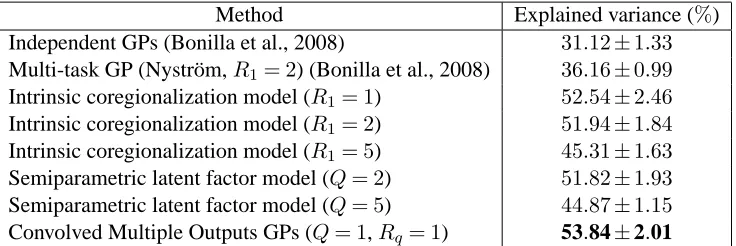
Train set Test set Method Average SMSE Average MSLL

Replica 1 Replica 2 LMC 0.6069±0.0294 −0.2687±0.0594

CMOC 0.4859±0.0387 −0.3617±0.0511

Replica 2 Replica 1 LMC 0.6194±0.0447 −0.2360±0.0696

CMOC 0.4615±0.0626 −0.3811±0.0748

Table 1: Standardized mean square error (SMSE) and mean standardized log loss (MSLL) for the

gene expression data for50outputs. CMOC stands for convolved multiple output

covari-ance. The experiment was repeated ten times with a different set of50 genes each time.

Table includes the value of one standard deviation over the ten repetitions. More negative values of MSLL indicate better models.

Table 1 shows the results of both methods over the test set for the two different replicas. It can be seen that the convolved multiple output covariance (appearing as CMOC in the table), outperforms the LMC covariance both in terms of SMSE and MSLL.

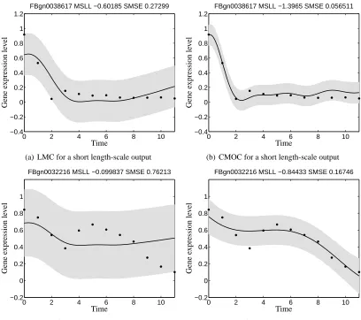
Figure 1 shows the prediction made over the test set (replica 2 in this case) by the two models for two particular genes, namely FBgn0038617 (Figure 1, first row) and FBgn0032216 (Figure 1, second row). The black dots in the figures represent the gene expression data of the particular genes. Figures 1(a) and 1(c) show the response of the LMC and Figures 1(b) and 1(d) show the response of the convolved multiple output covariance. It can be noticed from the data that the two genes differ in their responses to the action of the transcription factor, that is, while gene FBgn0038617 has

a rapid decay around time2and becomes relatively constant for the rest of the time interval, gene

FBgn0032216 has a smoother response within the time frame. The linear model of coregionalization is driven by a latent function with a length-scale that is shared across the outputs. Notice from Figures 1(a) and 1(c) that the length-scale for both responses is the same. On the other hand, due-to the non-instantaneous mixing of the latent function, the convolved multiple output framework, allows the description of each output using its own length-scale, which gives an added flexibility for describing the data.

Table 2 (first four rows) shows the performances of both models for the genes of Figure 1. CMOC outperforms the linear model of coregionalization for both genes in terms of SMSE and MSLL.

0 2 4 6 8 10 −0.4 −0.2 0 0.2 0.4 0.6 0.8 1 1.2

FBgn0038617 MSLL −0.60185 SMSE 0.27299

G ene expr es sion le v el Time

(a) LMC for a short length-scale output

0 2 4 6 8 10

−0.4 −0.2 0 0.2 0.4 0.6 0.8 1 1.2

FBgn0038617 MSLL −1.3965 SMSE 0.056511

G ene expr es sion le v el Time

(b) CMOC for a short length-scale output

0 2 4 6 8 10

−0.2 0 0.2 0.4 0.6 0.8 1

FBgn0032216 MSLL −0.099837 SMSE 0.76213

G ene expr es sion le v el Time

(c) LMC for a long length-scale output

0 2 4 6 8 10

−0.2 0 0.2 0.4 0.6 0.8 1

FBgn0032216 MSLL −0.84433 SMSE 0.16746

G ene expr es sion le v el Time

(d) CMOC for a long length-scale output

Figure 1: Predictive mean and variance for genes FBgn0038617 (first row) and FBgn0032216 (sec-ond row) using the linear model of coregionalization in Figures 1(a) and 1(c) and the

convolved multiple-output covariance in Figures 1(b) and 1(d), withQ= 1andRq= 1.

The training data comes from replica 1 and the testing data from replica 2. The solid line corresponds to the predictive mean, the shaded region corresponds to 2 standard devia-tions of the prediction. Performances in terms of SMSE and MSLL are given in the title of each figure and appear also in Table 2. The adjectives “short” and “long” given to the length-scales in the captions of each figure, must be understood like relative to each other.

Having said this, we can argue that the performance of the LMC model can be improved by

either increasing the value ofQor the valueRq, or both. For the intrinsic coregionalization model,

we would fix the value ofQ= 1and increase the value ofR1. Effectively, we would be increasing

the rank of the coregionalization matrix B1, meaning that more latent functions sampled from the

Test replica Test genes Method SMSE MSLL

Replica 2

FBgn0038617 LMC 0.2729 −0.6018

CMOC 0.0565 −1.3965

FBgn0032216 LMC 0.7621 −0.0998

CMOC 0.1674 −0.8443

Replica 1

FBgn0010531 LMC 0.2572 −0.5699

CMOC 0.0446 −1.3434

FBgn0004907 LMC 0.4984 −0.3069

CMOC 0.0971 −1.0841

Table 2: Standardized mean square error (SMSE) and mean standardized log loss (MSLL) for the genes in Figures 1 and 2 for LMC and CMOC. Genes FBgn0038617 and FBgn0010531 have a shorter length-scale when compared to genes FBgn0032216 and FBgn0004907.

of outputs, or in other words assuming a full rank for the matrix B1. This leads to the need of

estimating the matrix B1∈ ℜD×D, that might be problematic ifDis high. For the semiparametric

latent factor model, we would fix the value ofRq= 1and increaseQ, the number of latent functions

sampled from Qdifferent GPs. Again, in the extreme case of each output having its own

length-scale, we might need to estimate a matrixAe∈ ℜD×D_{, which could be problematic for a high value}

of outputs. In a more general case, we could also combine values ofQ >1andRq>1. We would

need then, to find values ofQandRqthat fit the different outputs with different length scales.

In practice though, we will see in the experimental section, that both the linear model of core-gionalization and the convolved multiple output GPs can perform equally well in some data sets. However, the convolved covariance could offer an explanation of the data through a simpler model or converge to the LMC, if needed.

5. Efficient Approximations for Convolutional Processes

Assuming that the double integral in Equation (8) is tractable, the principle challenge for the con-volutional framework is computing the inverse of the covariance matrix associated with the outputs.

ForDoutputs, each havingN data points, the inverse has computational complexityO(D3N3)and

associated storage ofO(D2_N2_{). We show how through making specific conditional independence}

assumptions, inspired by the model structure ( ´Alvarez and Lawrence, 2009), we arrive at a efficient

approximation similar in form to the partially independent training conditional model (PITC, see Qui˜nonero-Candela and Rasmussen, 2005). The relationship with PITC then inspires us to make further conditional independence assumptions.

5.1 Latent Functions as Conditional Means

For notational simplicity, we restrict the analysis of the approximations to one latent functionu(x). The key to all approximations is based on the form we assume for the latent functions. From the perspective of a generative model, Equation (7) can be interpreted as follows: first we draw a sample

from the Gaussian process priorp(u(z))and then solve the integral for each of the outputsfd(x)

0 2 4 6 8 10 −0.4 −0.2 0 0.2 0.4 0.6 0.8 1 1.2

FBgn0010531 MSLL −0.56996 SMSE 0.25721

G ene expr es sion le v el Time

(a) LMC for a short length-scale output

0 2 4 6 8 10

−0.4 −0.2 0 0.2 0.4 0.6 0.8 1 1.2

FBgn0010531 MSLL −1.3434 SMSE 0.044655

G ene expr es sion le v el Time

(b) CMOC for a short length-scale output

0 2 4 6 8 10

−0.1 −0.05 0 0.05 0.1 0.15 0.2 0.25 0.3

FBgn0004907 MSLL −0.30696 SMSE 0.49844

G ene expr es sion le v el Time

(c) LMC for a long length-scale output

0 2 4 6 8 10

−0.1 −0.05 0 0.05 0.1 0.15 0.2 0.25 0.3

FBgn0004907 MSLL −1.0841 SMSE 0.097131

G ene expr es sion le v el Time

(d) CMOC for a long length-scale output

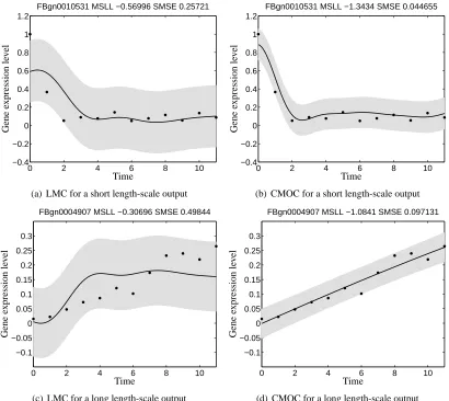
Figure 2: Predictive mean and variance for genes FBgn0010531 (first row) and FBgn0004907 (sec-ond row) using the linear model of coregionalization in Figures 2(a) and 2(c), and the

convolved multiple-output covariance in Figures 2(b) and 2(d), withQ= 1andRq= 1.

The difference with Figure 1 is that now the training data comes from replica 2 while the testing data comes from replica 1. The solid line corresponds to the predictive mean, the shaded region corresponds to 2 standard deviations of the prediction. Performances in terms of SMSE and MSLL are given in the title of each figure.

For the set of approximations, instead of drawing a sample fromu(z), we first draw a sample

from a finite representation ofu(z), u(Z) = [u(z1), . . . , u(zK)]⊤, where Z={zk}K_k=1is the set of

in-put vectors at whichu(z)is evaluated. Due to the properties of a Gaussian process,p(u(Z))follows

a multivariate Gaussian distribution. Conditioning on u(Z), we next sample from the conditional

priorp(u(z)|u(Z))and use this function to solve the convolution integral for eachfd(x).7 Under

this generative approach, we can approximate each functionfd(x)using

fd(x)≈ Z

X

Gd(x−z) E [u(z)|u]dz. (14)

Replacingu(z)forE [u(z)|u]is a reasonable approximation as long asu(z)is a smooth function

so that the infinite dimensional objectu(z) can be summarized by u. Figure 3 shows a cartoon

example of the quality of the approximations for two outputs as the size of the set Z increases. The first column represents the conditional priorp(u(z)|u)for a particular choice ofu(z). The second and third columns represent the outputsf1(x)andf2(x)obtained when using Equation (14).

Using expression (14), the likelihood function for f follows

p(f|u,Z,X,θ) =Nf|Kf,uKu−,1uu,Kf,f−Kf,uK−u,1uK⊤f,u

, (15)

where Ku,uis the covariance matrix between the samples from the latent function u(Z), with

ele-ments given byku,u(z,z′)and Kf,u=K⊤u,fis the cross-covariance matrix between the latent function u(z)and the outputsfd(x), with elementscov [fd(x), u(z)]in (9).

Given the set of points u, we can have different assumptions about the uncertainty of the out-puts in the likelihood term. For example, we could assume that the outout-puts are independent or uncorrelated, keeping only the uncertainty involved for each output in the likelihood term. Another approximation assumes that the outputs are deterministic, this is Kf,f=Kf,uKu−,1uK⊤f,u. The only

uncertainty left would be due to the priorp(u). Next, we present different approximations of the

covariance of the likelihood that lead to a reduction in computational complexity.

5.1.1 PARTIALINDEPENDENCE

We assume that the individual outputs in f are independent given the latent function u, leading to the following expression for the likelihood

p(f|u,Z,X,θ) = D Y

d=1

p(fd|u,Z,X,θ) = D Y

d=1

N f|Kfd,uK −1

u,uu,Kfd,fd−Kfd,uK −1 u,uKu,fd

.

We rewrite this product of multivariate Gaussians as a single Gaussian with a block diagonal co-variance matrix, including the uncertainty about the independent processes

p(y|u,Z,X,θ) =N y|Kf,uK−u,1uu,D+Σ

(16)

where D= blockdiaghKf,f−Kf,uK−u,1uK⊤f,u i

, and we have used the notationblockdiag [G]to

indi-cate that the block associated with each output of the matrix G should be retained, but all other elements should be set to zero. We can also write this as D=Kf,f−Kf,uK−u,1uKu,f

⊙M where

⊙ is the Hadamard product and M=ID⊗1N, 1N being theN×N matrix of ones. We now

marginalize the values of the samples from the latent function by using its process prior, this means

p(u|Z) =N(u|0,Ku,u). This leads to the following marginal likelihood,

p(y|Z,X,θ) = Z

p(y|u,Z,X,θ)p(u|Z)du=N y|0,D+Kf,uK−u,1uKu,f+Σ

−1 −0.8 −0.6 −0.4 −0.2 0 0.2 0.4 0.6 0.8 1 −2.5 −2 −1.5 −1 −0.5 0 0.5 1 1.5 2 2.5

(a) Conditional prior forK= 5

−1 −0.8 −0.6 −0.4 −0.2 0 0.2 0.4 0.6 0.8 1 −1 −0.5 0 0.5 1 1.5 2

(b) Output one forK= 5

−1 −0.8 −0.6 −0.4 −0.2 0 0.2 0.4 0.6 0.8 1 −1 −0.5 0 0.5 1 1.5 2

(c) Output two forK= 5

−1 −0.8 −0.6 −0.4 −0.2 0 0.2 0.4 0.6 0.8 1 −2.5 −2 −1.5 −1 −0.5 0 0.5 1 1.5 2 2.5

(d) Conditional prior forK= 10

−1 −0.8 −0.6 −0.4 −0.2 0 0.2 0.4 0.6 0.8 1 −1 −0.5 0 0.5 1 1.5 2

(e) Output one forK= 10

−1 −0.8 −0.6 −0.4 −0.2 0 0.2 0.4 0.6 0.8 1 −1 −0.5 0 0.5 1 1.5 2

(f) Output two forK= 10

−1 −0.8 −0.6 −0.4 −0.2 0 0.2 0.4 0.6 0.8 1 −2.5 −2 −1.5 −1 −0.5 0 0.5 1 1.5 2 2.5

(g) Conditional prior forK= 30

−1 −0.8 −0.6 −0.4 −0.2 0 0.2 0.4 0.6 0.8 1 −1 −0.5 0 0.5 1 1.5 2

(h) Output one forK= 30

−1 −0.8 −0.6 −0.4 −0.2 0 0.2 0.4 0.6 0.8 1 −1 −0.5 0 0.5 1 1.5 2

(i) Output two forK= 30

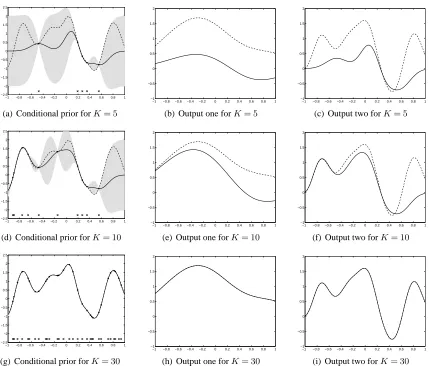
Figure 3: Conditional prior and two outputs for different values of K. The first column, Figures

3(a), 3(d) and 3(g), shows the mean and confidence intervals of the conditional prior distribution using one input function and two output functions. The dashed line represents one sample from the prior. Conditioning over a few points of this sample, shown as black dots, the conditional mean and conditional covariance are computed. The solid line represents the conditional mean and the shaded region corresponds to 2 standard deviations away from the mean. The second column, 3(b), 3(e) and 3(h), shows the solution to Equation (7) for output one using the sample from the prior (dashed line) and

the conditional mean (solid line), for different values ofK. The third column, 3(c), 3(f)

and 3(i), shows the solution to Equation (7) for output two, again for different values of

K.

Notice that, compared to (13), the full covariance matrix Kf,fhas been replaced by the low rank

co-variance Kf,uK−u,1uKu,fin all entries except in the diagonal blocks corresponding to Kfd,fd.

Depend-ing on our choice ofK, the inverse of the low rank approximation to the covariance is either

Note that if we setK=N these reduce toO(N3_D)andO(N2_{D)respectively. Rather neatly this}

matches the computational complexity of modeling the data withDindependent Gaussian processes

across the outputs.

The functional form of (17) is almost identical to that of the partially independent training conditional (PITC) approximation (Qui˜nonero-Candela and Rasmussen, 2005) or the partially inde-pendent conditional (PIC) approximation (Qui˜nonero-Candela and Rasmussen, 2005; Snelson and Ghahramani, 2007), with the samples we retain from the latent function providing the same role as

the inducing values in the PITC or PIC.8 This is perhaps not surprising given that the PI(T)C

ap-proximations are also derived by making conditional independence assumptions. A key difference is that in PI(T)C it is not obvious which variables should be grouped together when making these conditional independence assumptions; here it is clear from the structure of the model that each of the outputs should be grouped separately.

5.1.2 FULLINDEPENDENCE

We can be inspired by the analogy of our approach to the PI(T)C approximation and consider a more radical factorization of the likelihood term. In the fully independent training conditional (FITC) ap-proximation or the fully independent conditional (FIC) apap-proximation (Snelson and Ghahramani, 2006, 2007), a factorization across the data points is assumed. For us that would lead to the follow-ing expression for the conditional distribution of the output functions given the inducfollow-ing variables,

p(f|u,Z,X,θ) = D Y

d=1 N Y

n=1

p(fn,d|u,Z,X,θ),

which can be expressed through (16) with D= diaghKf,f−Kf,uK−u,1uK⊤f,u i

=hKf,f−Kf,uK−u,1uK⊤f,u i

⊙ M, with M=ID⊗INor simply M=IDN. The marginal likelihood, including the uncertainty about

the independent processes, is given by Equation (17) with the diagonal form for D. Training with

this approximated likelihood reduces computational complexity toO(K2DN)and the associated

storage toO(KDN).

5.1.3 DETERMINISTICLIKELIHOOD

In Qui˜nonero-Candela and Rasmussen (2005), the relationship between the projected process ap-proximation (Csat´o and Opper, 2001; Seeger et al., 2003) and the FI(T)C and PI(T)C approxima-tions is elucidated. They show that if, given the set of values u, the outputs are assumed to be deterministic, the likelihood term of Equation (15) can be simplified as

p(f|u,Z,X,θ) =N f|Kf,uK−u,1uu,0

.

Marginalizing with respect to the latent function using p(u|Z) =N(u|0,Ku,u) and including the

uncertainty about the independent processes, we obtain the marginal likelihood as

p(y|Z,X,θ) = Z

p(y|u,Z,X,θ)p(u|Z)du=Ny|0,Kf,uKu−,1uK⊤f,u+Σ

.

In other words, we can approximate the full covariance Kf,f using the low rank approximation

Kf,uK−u,1uK⊤f,u. Using this new marginal likelihood to estimate the parametersθ reduces

computa-tional complexity toO(K2_{DN). The approximation obtained has similarities with the projected}

latent variables (PLV) method also known as the projected process approximation (PPA) or the de-terministic training conditional (DTC) approximation (Csat´o and Opper, 2001; Seeger et al., 2003; Qui˜nonero-Candela and Rasmussen, 2005; Rasmussen and Williams, 2006).

5.1.4 ADDITIONALINDEPENDENCEASSUMPTIONS

As mentioned before, we can consider different conditional independence assumptions for the like-lihood term. One further assumption that is worth mentioning considers conditional independencies across data points and dependence across outputs. This would lead to the following likelihood term

p(f|u,Z,X,θ) = N Y

n=1

p(fn|u,Z,X,θ),

where fn= [f1(xn), f2(xn), . . . , fD(xn)]⊤. We can use again Equation (16) to express the likelihood.

In this case, though, the matrix D is a partitioned matrix with blocks Dd,d′∈ ℜN×N and each block

Dd,d′ would be given as D_d,d′ = diag

Kfd,fd′−Kfd,uK −1 u,uKu,f_d′

. For cases in which D > N, that is, the number of outputs is greater than the number of data points, this approximation may be more

accurate than the one obtained with the partial independence assumption. For cases whereD < N

it may be less accurate, but faster to compute.9

5.2 Posterior and Predictive Distributions

Combining the likelihood term for each approximation withp(u|Z)using Bayes’ theorem, the

pos-terior distribution over u is obtained as

p(u|y,X,Z,θ) =N u|Ku,uA−1Ku,f(D+Σ)−1y,Ku,uA−1Ku,u

, (18)

where A=Ku,u+K⊤_f,u(D+Σ)−1Kf,u and D follows a particular form according to the different

approximations: for partial independence it equals D= blockdiagKf,f−Kf,uK−u,1uKu,f

; for full independence it is D= diagKf,f−Kf,uK−u,1uKu,f

and for the deterministic likelihood, D=0.

For computing the predictive distribution we have two options, either use the posterior for u and the approximated likelihoods or the posterior for u and the likelihood of Equation (15), that cor-responds to the likelihood of the model without any approximations. The difference between both options is reflected in the covariance for the predictive distribution. Qui˜nonero-Candela and Ras-mussen (2005) proposed a taxonomy of different approximations according to the type of likelihood used for the predictive distribution, in the context of single output Gaussian processes.

In this paper, we opt for the posterior for u and the likelihood of the model without any approx-imations. If we choose the exact likelihood term in Equation (15) (including the noise term), the

9. Notice that if we work with the block diagonal matrices Dd,d′, we would need to invert the full matrix D. However,

since the blocks Dd,d′are diagonal matrices themselves, the inversion can be done efficiently using, for example, a

predictive distribution is expressed through the integration of the likelihood term evaluated at X∗,

with (18), giving

p(y∗|y,X,X∗,Z,θ) = Z

p(y∗|u,Z,X∗,θ)p(u|y,X,Z,θ)du=N(y∗|µy∗,Ky∗,y∗),

where

µy∗=Kf∗,uA

−1_K⊤

f,u(D+Σ)−1y,

Ky∗,y∗=Kf∗,f∗−Kf∗,uK

−1

u,uK⊤f∗,u+Kf∗,uA

−1_K⊤

f∗,u+Σ∗.

For the single output case, the assumption of the deterministic likelihood is equivalent to the de-terministic training conditional (DTC) approximation, the full independence approximation leads to the fully independent training conditional (FITC) approximation (Qui˜nonero-Candela and Ras-mussen, 2005) and the partial independence leads to the partially independent training conditional (PITC) approximation (Qui˜nonero-Candela and Rasmussen, 2005). The similarities of our approx-imations for multioutput GPs with respect to approxapprox-imations presented in Qui˜nonero-Candela and Rasmussen (2005) for single output GPs are such, that we find it convenient to follow the same terminology and also refer to our approximations as DTC, FITC and PITC approximations for mul-tioutput Gaussian processes.

5.3 Discussion: Model Selection in Approximated Models

The marginal likelihood approximation for the PITC, FITC and DTC variants is a function of both the hyperparameters of the covariance function and the location of the inducing variables. For es-timation purposes, there seems to be a consensus in the GP community that hyperparameters for the covariance function can be obtained by maximization of the marginal likelihood. For selecting the inducing variables, though, there are different alternatives that can in principle be used. Simpler methods include fixing the inducing variables to be the same set of input data points or grouping

the input data using a clustering method likeK-means and then use theK resulting vectors as

in-ducing variables. More sophisticated alternatives consider that the set of inin-ducing variables must be restricted to be a subset of the input data (Csat´o and Opper, 2001; Williams and Seeger, 2001). This set of methods require a criteria for choosing the optimal subset of the training points (Smola and Bartlett, 2001; Seeger et al., 2003). Such approximations are truly sparse in the sense that only few data points are needed at the end for making predictions. Recently, Snelson and Ghahramani (2006) suggested using the marginal likelihood not only for the optimization of the hyperparameters in the covariance function, but also for the optimization of the location of these inducing variables. Although, using such procedure to find the optimal location of the inducing inputs might look in principle like an overwhelming optimization problem (inducing points usually appear non-linearly in the covariance function), in practice it has been shown that performances close to the full GP model can be obtained in a fraction of the time that it takes to train the full model. In that re-spect, the inducing points that are finally found are optimal in the same optimality sense that the hyperparameters of the covariance function.

In appendix A we include the derivatives of the marginal likelihood wrt the matrices Kf,f,Ku,f

and Ku,u.

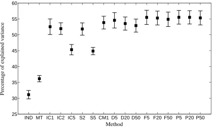
6. Experimental Evaluation

In this section we present results of applying the approximations in exam score prediction, pol-lutant metal prediction and the prediction of gene expression behavior in a gene-network. When possible, we first compare the convolved multiple output GP method against the intrinsic model of coregionalization and the semiparametric latent factor model. Then, we compare the different approximations in terms of accuracy and training times. First, though, we illustrate the performance

of the approximation methods in a toy example.10

6.1 A Toy Example

For the toy experiment, we employ the kernel constructed as an example in Section 3. The toy

problem consists ofD= 4outputs, one latent function,Q= 1andRq= 1and one input dimension.

The training data was sampled from the full GP with the following parameters, S1,1=S2,1 = 1,

S3,1=S4,1= 5, P1,1 =P2,1 = 50, P3,1= 300, P4,1= 200 for the outputs andΛ1 = 100for the

latent function. For the independent processes,wd(x), we simply added white noise separately to

each output so we have variancesσ₁2=σ2₂= 0.0125,σ2₃= 1.2andσ2₄= 1. We generateN = 500

observation points for each output and use200observation points (per output) for training the full

and the approximated multiple output GP and the remaining300observation points for testing. We

repeated the same experiment setup ten times and compute the standardized mean square error and

the mean standardized log loss. For the approximations we useK= 30inducing inputs. We sought

the kernel parameters and the positions of the inducing inputs through maximizing the marginal likelihood using a scaled conjugate gradient algorithm. Initially the inducing inputs are equally spaced between the interval[−1,1].

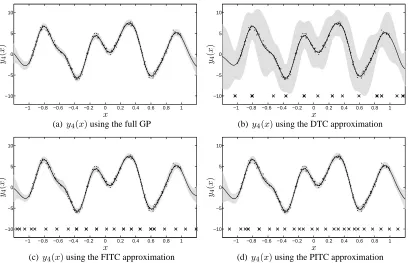
Figure 4 shows the training result of one of the ten repetitions. The predictions shown corre-spond to the full GP in Figure 4(a), the DTC approximation in Figure 4(b), the FITC approximation in Figure 4(c) and the PITC approximation in Figure 4(d).

Tables 3 and 4 show the average prediction results over the test set. Table 3 shows that the SMSE of the approximations is similar to the one obtained with the full GP. However, there are important differences in the values of the MSLL shown in Table 4. DTC offers the worst performance. It gets better for FITC and PITC since they offer a more precise approximation to the full covariance.

The training times for iteration of each model are1.97secs for the full GP,0.20secs for DTC,

0.41for FITC and0.59for the PITC, on average.

As we have mentioned before, one important feature of multiple output prediction is that we can exploit correlations between outputs to predict missing observations. We used a simple example to

illustrate this point. We removed a portion of one output between[−0.8,0]from the training data in

the experiment before (as shown in Figure 5) and train the different models to predict the behavior of

y4(x)for the missing information. The predictions shown correspond to the full GP in Figure 5(a),

an independent GP in Figure 5(b), the DTC approximation in Figure 5(c), the FITC approximation in

−1 −0.8 −0.6 −0.4 −0.2 0 0.2 0.4 0.6 0.8 1 −10

−5 0 5 10

y4

(

x

)

x

(a)y₄(x)using the full GP

−1 −0.8 −0.6 −0.4 −0.2 0 0.2 0.4 0.6 0.8 1

−10 −5 0 5 10

y4

(

x

)

x

(b)y₄(x)using the DTC approximation

−1 −0.8 −0.6 −0.4 −0.2 0 0.2 0.4 0.6 0.8 1

−10 −5 0 5 10

y4

(

x

)

x

(c)y₄(x)using the FITC approximation

−1 −0.8 −0.6 −0.4 −0.2 0 0.2 0.4 0.6 0.8 1

−10 −5 0 5 10

y4

(

x

)

x

(d) y₄(x)using the PITC approximation

Figure 4: Predictive mean and variance using the full multi-output GP and the approximations for output 4. The solid line corresponds to the predictive mean, the shaded region

corre-sponds to 2 standard deviations of the prediction. The dashed line corresponds to the

ground truth signal, that is, the sample from the full GP model without noise. In these plots the predictive mean overlaps almost exactly with the ground truth. The dots are the noisy training points. The crosses in Figures 4(b), 4(c) and 4(d) correspond to the locations of the inducing inputs after convergence. Notice that the DTC approximation in Figure 4(b) captures the predictive mean correctly, but fails in reproducing the correct predictive variance.

Method SMSEy1(x) SMSEy2(x) SMSEy3(x) SMSEy4(x)

Full GP 1.06±0.08 0.99±0.06 1.10±0.09 1.05±0.09

DTC 1.06±0.08 0.99±0.06 1.12±0.09 1.05±0.09

FITC 1.06±0.08 0.99±0.06 1.10±0.08 1.05±0.08

PITC 1.06±0.08 0.99±0.06 1.10±0.09 1.05±0.09

Table 3: Standardized mean square error (SMSE) for the toy problem over the test set. All numbers

are to be multiplied by10−2_{. The experiment was repeated ten times. Table includes the}

value of one standard deviation over the ten repetitions.

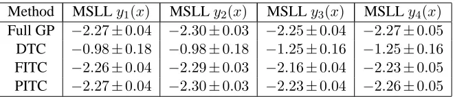
Method MSLLy1(x) MSLLy2(x) MSLLy3(x) MSLLy4(x)

Full GP −2.27±0.04 −2.30±0.03 −2.25±0.04 −2.27±0.05

DTC −0.98±0.18 −0.98±0.18 −1.25±0.16 −1.25±0.16

FITC −2.26±0.04 −2.29±0.03 −2.16±0.04 −2.23±0.05

PITC −2.27±0.04 −2.30±0.03 −2.23±0.04 −2.26±0.05

Table 4: Mean standardized log loss (MSLL) for the toy problem over the test set. More negative values of MSLL indicate better models. The experiment was repeated ten times. Table includes the value of one standard deviation over the ten repetitions.

Due to the strong dependencies between the signals, our model is able to capture the correlations and predicts accurately the missing information.

6.2 Exam Score Prediction

In the first experiment with real data that we consider, the goal is to predict the exam score obtained by a particular student belonging to a particular school. The data comes from the Inner London

Education Authority (ILEA).11 It consists of examination records from 139 secondary schools in

years 1985, 1986 and 1987. It is a random 50% sample with 15362 students. The input space

consists of four features related to each student (year in which each student took the exam, gender,

performance in a verbal reasoning (VR) test12 _{and ethnic group) and four features related to each}

school (percentage of students eligible for free school meals, percentage of students in VR band one, school gender and school denomination). From the multiple output point of view, each school represents one output and the exam score of each student a particular instantiation of that output or

D= 139.

We follow the same preprocessing steps employed in Bonilla et al. (2008). The only features used are the student-dependent ones, which are categorial variables. Each of them is transformed to a binary representation. For example, the possible values that the variable year of the exam can

take are 1985, 1986 or 1987 and are represented as 100, 010or 001. The transformation is also

applied to the variables gender (two binary variables), VR band (four binary variables) and ethnic

group (eleven binary variables), ending up with an input space with20dimensions. The categorial

nature of the data restricts the input space toN = 202unique input feature vectors. However, two

students represented by the same input vector x, and belonging both to the same school,d, can obtain

different exam scores. To reduce this noise in the data, we take the mean of the observations that, within a school, share the same input vector and use a simple heteroskedastic noise model in which

the variance for each of these means is divided by the number of observations used to compute it.13

The performance measure employed is the percentage of explained variance defined as the total variance of the data minus the sum-squared error on the test set as a percentage of the total data variance. It can be seen as the percentage version of the coefficient of determination between the

11. This data is available at http://www.cmm.bristol.ac.uk/learning-training/multilevel-m-support/ datasets.shtml.

12. Performance in the verbal reasoning test was divided in three bands. Band 1 corresponds to the highest25%, band 2 corresponds to the next50%and band 3 the bottom25%(Nuttall et al., 1989; Goldstein, 1991).