Matrix Completion with the Trace Norm:
Learning, Bounding, and Transducing
Ohad Shamir [email protected]
Department of Computer Science and Applied Mathematics Weizmann Institute of Science
Rehovot 7610001, Israel
Shai Shalev-Shwartz [email protected]
School of Computer Science and Engineering The Hebrew University
Givat Ram, Jerusalem 9190401, Israel
Editor:Tommi Jaakkola
Abstract
Trace-norm regularization is a widely-used and successful approach for collaborative fil-tering and matrix completion. However, previous learning guarantees require strong as-sumptions, such as a uniform distribution over the matrix entries. In this paper, we bridge this gap by providing such guarantees, under much milder assumptions which correspond to matrix completion as performed in practice. In fact, we claim that previous difficulties partially stemmed from a mismatch between the standard learning-theoretic modeling of matrix completion, and its practical application. Our results also shed some light on the issue of matrix completion with bounded models, which enforce predictions to lie within a certain range. In particular, we provide experimental and theoretical evidence that such models lead to a modest yet significant improvement.
Keywords: collaborative filtering, matrix completion, trace-norm regularization, trans-ductive learning, sample complexity
1. Introduction
We consider the problem of matrix completion, where the goal is to predict entries of an unknown matrix based on a subset of its observed entries. A popular approach to achieve this is via trace-norm regularization, where one seeks a matrix that agrees well with the observed entries, while constraining its complexity in terms of the norm. The trace-norm is well-known to be a convex surrogate to the matrix rank, and has repeatedly shown good performance in practice (Srebro et al., 2004; Salakhutdinov and Mnih, 2007; Bach, 2008; Cand`es and Tao, 2009).
distri-bution of ratings differ drastically between users. Modeling such data as a uniform sample is not a reasonable assumption. Another paper (Negahban and Wainwright, 2010) studied the problem of matrix completion under a non-uniform distribution. However, the analy-sis is still not distribution-free, and requires strong assumptions on the underlying matrix. Moreover, the results do not apply to standard trace-norm regularization, but rather to a carefully re-weighted version of trace-norm regularization.
In practice, we know that standard trace-norm regularization works quite well even for data which is very non-uniform. Moreover, we know that in other learning problems, one is able to derive distribution-free guarantees, and there is no a-priori reason why this should not be possible here. Nevertheless, obtaining a non-trivial guarantee for trace-norm regularization has remained elusive. This partially motivated work on alternative complexity measures for matrix completion, such as the max-norm and weighted variants of the trace-norm (see further discussion below).
In this paper, we bridge this gap between our theoretical understanding and practical performance of trace-norm regularization. We show that by adding very mild assumptions, which correspond to matrix completion as performed in practice, it is possible to learn in a distribution-free manner by observing O(n3/2) entries from an m×n matrix (where
m ≤ n, and for a reasonable trace-norm regime). Moreover, this bound is tight. When
m= Θ(n), this corresponds to viewing a vanishingly small portion of the entries, hence we get a non-trivial learning guarantee. In fact, we claim that the difficulties in providing such guarantees partially stemmed from a mismatch between the standard theoretical modeling of matrix completion, and its practical application. We emphasize that our bounds are weaker than previous bounds in the literature, which required observing as few as ˜O(n) entries (up to log factors). However, these bounds hold only under restrictive distributional assumptions, whereas our bounds hold under any distribution, and are provably tight in such a distribution-free setting.
First, we show that one can obtain such guarantees, if one takes into account that the values to be predicted are bounded. For example, in predicting movie ratings, it is known in advance that the ratings are on a scale of (say) 1 to 5, and practitioners usually clip their predictions to be inside this range. While this seems like an almost trivial operation, we show that taking it into account has far-reaching implications in terms of the theoretical guarantees. The proof relies on a decomposition technique which might also be useful for regularizers other than the trace-norm.
Second, we argue that the standardinductive model of learning, where the training data is assumed to be sampled i.i.d. from some distribution, may not be the best way to analyze matrix completion. Instead, we look at the transductive model, where sampling of the data is done without replacement. In the context of matrix completion, we show this makes a large difference in terms of the attainable guarantees.
which appeared since the preliminary version of this paper was published, relate to and strengthen our observations.
The paper is structured as follows. We begin by describing the setting and the notation we use in Section 2, and introduce the sample complexity issues of matrix completion with the trace norm in Section 3. In Section 4, we show how we can non-trivially learn with the trace-norm in an inductive i.i.d. setting, under boundedness assumptions. In Section 5, we show how similar performance can be ensured if we switch from an inductive setting to a transductive setting, where each entry appears only once in the data. We provide matching lower bounds in Section 6. In Section 7, we experimentally investigate how boundedness assumptions affect practical performance. Section 8 contains a discussion of how some recent works relate to our paper, and Section 9 contains full proofs of our results. We end with a discussion and some open issues in Section 10.
2. Setting
Our goal is to predict entries of an unknown m×n matrix X, based on a random subset of observed entries of X. A common way to achieve this, following standard learning approaches, is to find an m×n matrix W from a constrained class of matrices W, which minimizes the discrepancy from X on the observed entries. More precisely, if we let S =
{iα, jα}denote the set of (row,column) observed entries, and`is a loss function measuring the discrepancy between the predicted and actual value, then we solve the optimization problem
min W∈W
1
|S| |S|
X
α=1
`(Wiα,jα, Xiα,jα), (1)
An important and widely used class of matrices W are those with boundedtrace-norm
(sometimes also denoted as the nuclear norm or the Ky-Fann norm). Given a matrix W, its trace-normkWktr is defined as the sum of the singular values. The class of matrices with bounded trace-norm has several useful properties, such as it being a convex approximation of class of rank-bounded matrices (e.g., Srebro and Shraibman, 2005). Thus, we can often optimize Equation (1) in a computationally tractable manner, learning predictors which are competitive with low-rank matrices. The trace-norm of any m×n matrix W is at least kWkF and at most Rank(W)kWkF, where kWkF is the Frobenius norm (Horn and Johnson, 1985), and therefore the trace-norm of constant-rankm×nmatrices with bounded entries is Θ(√mn). Therefore, we wish to attain learning guarantees which are non-trivial when the trace norm is at least on the order of t= Θ(√mn). However, our theorems will hold for anyt.
For now, we will consider the inductive model of learning, which parallels the standard agnostic-PAC learnability framework. The model is defined as follows: We assume there exists an unknown distribution D over {1, . . . , m} × {1, . . . , n}. Each instantiation (i, j) provides the value Xi,j of an entry at a randomly picked row i and column j. An i.i.d. sample S = {iα, jα} of indices is chosen, and the corresponding entries {Xiα,jα} are
re-vealed. Our goal is to find a matrix W ∈ W such that its risk (or generalization error),
Equa-tion (1), if we can provide a non-trivial uniform sample complexity bound, namely a bound on
sup W∈W
Ei,j[`(Wi,j, Xi,j)]− 1
|S| |S|
X
α=1
`(Wiα,jα, Xiα,jα)
. (2)
A major focus of this paper is studying the difficulties and possibilities of obtaining such bounds.
3. Sample Complexity Bounds for the Trace-Norm
Consider the class of trace-norm constrained matrices, W = {W :kWktr ≤t}. Although learning with respect to this class is widely used in matrix completion, understanding its generalization and sample-complexity properties has proven quite elusive. Sample complex-ity bounds of the form O(p(m+n)/|S|) (when t = Θ(√mn), and ignoring logarithmic factors) were obtained under the strong assumption of a uniform distribution over the ma-trix entries (Srebro and Shraibman, 2005). However, this assumption does not correspond to real-world matrix completion data sets, where the distribution of the revealed entries appears to be highly non-uniform. Other works, which focused on exact matrix completion (e.g., Cand`es and Tao, 2009; Cand`es and Recht, 2009), also assume a uniform sampling distribution.
The bounds in Srebro and Shraibman (2005) are based on the Rademacher complexity of the classW, and will be utilized in our analysis as well. Formally, we define the (empirical) Rademacher complexity of a hypothesis class W combined with a loss function `, with respect to a sampleS, as
RS(`◦ W) =Eσ
sup
W∈W
1
|S| |S|
X
α=1
σα`(Wiα,jα, Xiα,jα)
, (3)
where σ1, . . . , σ|S| are i.i.d. random variables taking the values −1 and +1 with equal
probability.
Rademacher complexities play a key role in obtaining sample complexity bounds, ei-ther in expectation or in high probability. The following is a typical example (based on Boucheron and Lugosi, 2005, Theorem 3.2):
Theorem 1 The expected value of Equation (2) is at most2RS(`◦W). Moreover, if there is
a constant b` such thatsupi,j,W∈W|`(Wi,j, Xi,j)| ≤b`, then for any δ∈(0,1), Equation (2)
is bounded with probability at least 1−δ by 2RS(`◦ W) +b`
p
2 log(2/δ)/|S|.
In general, the dominant term in the bound above is the Rademacher complexityRS(`◦W). Thus, if we can upper-bound the Rademacher complexity by a quantity much smaller than 1, we get a non-trivial upper bound on Equation (2). Such a bound implies that the empirical risk (or average loss over the training set) is close to the true risk uniformly for allW ∈ W, and therefore that solving Equation (1) will lead to a predictor with near-optimal risk.
way to analyze Equation (3) (see Bartlett and Mendelson, 2003) is to use the contraction principle to upper bound it by
Eσ
sup
W∈W
1
|S| |S|
X
α=1
σαWiα,jα
,
and then using H¨older’s inequality to upper bound it by
Eσ
sup W∈W
1
|S|kΓkspkWktr
= t 1
|S|E[kΓksp],
where Γ is a matrix whose (i, j)-th entry is defined as P
α:iα=i,jα=jσα, and k · ksp is the
spectral norm (i.e., the largest singular value), which is well-known to be dual to the trace-norm (Fazel et al., 2001). However, if for instance all σα are on the same entry i, j, then
E[kΓksp] equals E[|Pασα|] = Θ(
p
|S|), leading to a bound of the form O(t/p|S|). As discussed earlier, tis typically at least on the order of√mn, in which case we get a bound on the Rademacher complexity which is O(pmn/|S|) — smaller than 1 only when the sample size |S| is larger than the total numbermn of matrix entries. It is a trivial bound, since the entire goal of matrix completion is prediction based on observing just a small subset of the matrix entries.
Unfortunately, this bound appears impossible to improve in general (see section 6.2.2 in Srebro, 2004). Srebro and Shraibman (2005) circumvent this by imposing a strong uniform distribution assumption, under which a tighter bound is attainable. The main drive of our paper is that by modifying the setting in some very simple ways, which often correspond to matrix completion as done in practice, one can obtain non-trivial learning guarantees without any distributional assumptions.
4. Results for the Inductive Model
In this section, we show that by introducingboundedness conditions into the learning prob-lem, one can obtain non-trivial bounds on the Rademacher complexity, and hence on the sample complexity of learning with trace-norm constraints.
We will start with the case where we actually learn with respect to the hypothesis class of trace-norm-constrained matrices, W ={W :kWktr ≤t}, and the only boundedness is in terms of the loss function:
Theorem 2 Consider the hypothesis class W = {W : kWktr ≤ t}. Suppose that for all i, j the loss function `(·, Xi,j) is both b`-bounded and l`-Lipschitz in its first argument:
Namely, that `(Wi,j, Xi,j)≤b` for any W, i, j, and that
|`(Wi,j,Xi,j)−`(Wi,j0 ,Xi,j)|
|Wi,j−Wi,j0 |
≤l` for any
W, W0, i, j. Then
RS(`◦ W)≤
s
9Cl`b`
t(√m+√n)
When t= Θ(√mn), the theorem implies that a sample of size O(n√m+m√n) is suffi-cient to obtain good generalization performance. We note that the boundedness assumption is non-trivial, since the trace-norm constraint does not imply entries of constant magnitude (the entries can be as large astfor a matrix whose trace norm is t). On the other hand, as discussed earlier, the obtainable bound on the Rademacher complexity without a bound-edness assumption is no better than O((m+n)/p|S|), which leads to a trivial required sample size ofO((m+n)2). Moreover, we emphasize that the result makes no assumptions on the underlying distribution from which the data was sampled. The proof is presented in Subsection 9.1. We note that it relies on a decomposition technique which might also be useful for regularizers other than the trace-norm.
An alternative way to introduce boundedness, and get a non-trivial guarantee, is by composing the entries of a matrix W with a bounded transfer function. In particular, rather than just learning a matrix W with bounded trace-norm, we can learn a model
φ◦W, where W has bounded trace-norm, and φ:R7→I is a fixed mapping of each entry
ofW into some bounded intervalI ⊆R. This model is used in practice, and is useful in the common situation where the entries ofX are known to be in a certain bounded interval. In Section 7, we return to this model in greater depth. In terms of the theoretical guarantee, one can provide a result similar to Theorem 2, without assuming boundedness of the loss function.
Theorem 3 Consider the hypothesis classW ={φ◦W :kWktr ≤t}. Letφ:R7→[−bφ, bφ]
be a bounded lφ-Lipschitz function, and suppose that for all i, j, `(·, Xi,j) isl`-Lipschitz on
the domain [−bφ, bφ]. Then
RS(`◦ W)≤l`
s
9Clφbφ
t(√m+√n)
|S| , where C is the universal constant appearing in Theorem 8.
The bound in this theorem scales similarly to Theorem 2, in terms of its dependence on
m, n. Another possible variant is directly learning a matrix W with both a constraint on the trace-norm, as well as an ∞-norm constraint (i.e., maxi,j|Wi,j| ≤c for some constant
c) which forces the matrix entries to be constant. This model has some potential benefits which shall be further discussed in Section 10.
Theorem 4 Consider the hypothesis class W = {W : kWktr ≤ t,kWk∞ ≤ b}, where kWk∞ = maxi,j|Wi,j|. Suppose that for all i, j, `(·, Xi,j) is l`-Lipschitz on the domain [−b, b]. Then
RS(`◦ W)≤l`
s
9Cbt( √
n+√m)
|S| , where C is the universal constant appearing in Theorem 8.
Assuming b is a constant (which is the reasonable assumption here), we get a similar bound as before.
constraints. These were all obtained under the standard inductive model, where we assume that our data is an i.i.d. sample from an underlying distribution. In the next section, we will discuss a different learning model, which we argue to more closely resemble matrix completion as done in practice, and leads to better bounds on the Rademacher complexity, without making boundedness assumptions.
5. Improved Results for the Transductive Model
In the inductive model we have considered so far, the goal is to predict well with respect to an unknown distribution over matrix entries, given an i.i.d. sample from that distribution. The transductive learning model (see for instance Vapnik, 1998) is different, in that our goal is to predict well with respect to aspecific subset of entries, whose location is known in advance. More formally, we fix an arbitrary subset ofS entries, and then split it uniformly at random into two subsets Strain ∪Stest. We are then given the values of the entries in
Strain, and our goal is to predict the values of the entries in Stest. For simplicity, we will assume that |Strain| = |Stest| = |S|/2, but our results can be easily generalized to more general partitions.
We note that this procedure isexactly the one often performed in experiments reported in the literature: Given a data set of entries, one randomly splits it into a training set and a test set, learns a matrix on the training set, and measures its performance on the test set (e.g., Toh and Yun, 2009; Jaggi and Sulovsk´y, 2010). Even for other train-test split methods, such as holding out a certain portion of entries from each row, the transductive model seems closer to reality than the inductive model. Moreover, the transductive model captures another important feature of real-world matrix completion: the fact that no entry is repeated in the training set. In contrast, in the inductive model the training set is collected i.i.d., so the same entry might be sampled several time over. In fact, this is virtually certain to happen whenever the sample size is at least on the order of √mn, due to the birthday paradox. This does not appear to be a mere technicality, since the proofs of our theorems in the inductive model have to rely on a careful separation of the entries according to the number of times they were sampled. However, in reality each entry appears in the data set only once, matching the transductive learning setting.
To analyze the transductive model, we require analogues of the tools we have for the inductive model, such as the Rademacher complexity. Fortunately, such analogues were al-ready obtained in the literature (El-Yaniv and Pechyoni, 2009), and we will rely on their re-sults. In particular, based on Theorem 1 in that paper, we can use our notion of Rademacher complexity, as defined in Equation (3), to provide sample complexity bounds in the trans-ductive model:1
Theorem 5 Fix a hypothesis classW, and suppose thatsupi,j,W∈W|`(Wi,j, Xi,j)| ≤b`. Let
a set S of ≥ 2 distinct indices be fixed, and suppose it is uniformly and randomly split to two equal subsets Strain, Stest. Then with probability at least 1−δ over the random split, it
1. In El-Yaniv and Pechyoni (2009), a more general notion of transductive Rademacher complexity was defined, where theσα random variables could also take 0 values. However, when|Strain|=|Stest|, that
holds for any W ∈ W that
1
|Stest|
X
(i,j)∈Stest
`(Wi,j, Xi,j)− 1
|Strain|
X
(i,j)∈Strain
`(Wi,j, Xi,j)
≤4RS(`◦ W) +
b`
11 + 4plog(1/δ)
p
|Strain|
.
This theorem implies that if RS(`◦ W) is effectively bounded, then the average loss over
Strain is close to the average loss overStest, uniformly for anyW, and therefore minimizing the average loss over Strain will result in a predictor with near-optimal average loss over
Stest.
We now present our main result for the transductive model, which implies non-trivial bounds on the Rademacher complexity of matrices with constrained trace-norm. Unlike the inductive model, here we make no additional boundedness assumptions, yet the bound is superior. The proof appears in Subsection 9.4.
Theorem 6 Consider the hypothesis classW ={W :kWktr ≤t}. Then in the transductive
model, it holds that
RS(`◦ W)≤Cl`
3t(√m+√n) 2|S| ,
where C is the universal constant appearing in Theorem 8. Alternatively, letting N = maxi|{j: (i, j)∈S}|and M = maxj|{i: (i, j)∈S}|, then
RS(`◦ W)≤Cl`
t maxn√M ,√No |S|
4
p
log(min{m, n}),
where C is the universal constant appearing in Theorem 9.
We note that the second bound, while containing an additional logarithmic term, de-pends on the distribution of the entries, and can be considerably tighter than the worst-case. To see this, suppose (for simplicity) a rectangular matrix, so that m = n, and that t = Θ(√mn) = Θ(n). Then in the worst-case, the bound becomes meaningful when
|S| = Ω(n3/2). However, if the entries in S are (approximately) uniformly distributed throughout the matrix, then the maximal number of entries in each row and column is
O(|S|/n). In that case, plugging|S|/ninstead ofM and N, as well ast= Θ(n), we obtain the bound
RS(`◦ W)≤O˜
r n
|S|
(ignoring logarithmic factors), which is already meaningful when|S|= ˜Ω(n). Interestingly, this bound is similar (up to logarithmic factors) to previous bounds in the inductive setting (e.g., Srebro and Shraibman, 2005)), which relied on a uniform distribution assumption. However, our Rademacher complexity bound in Theorem 6 also applies to non-uniform distributions, and is meaningful for any distribution.
factor does appear in a different term in the cited overall sample complexity bound (The-orem 5), we conjecture that its true effect is modest at best. This is in light of recent work, which imply that using particular online matrix completion algorithms, one can learn comparatively well in a transductive setting, without explicit boundedness assumptions (see Section 8).
Another interesting feature of Theorem 6 is that the Rademacher complexity falls off at the rate of O(1/|S|) rather than O(1/p|S|). While such a “fast rate” is unusual in the inductive setting, here it is a natural outcome of the different modeling of the training data. This does not lead to a O(1/|S|) sample complexity bound, because the bound in Theorem 5 contains an additional low rate term O(1/p|S|). However, it still leads to a better bound because the low rate term is not explicitly multiplied by functions ofm, n or
t.
6. Lower Bounds
The previous results showed that for m×n matrices (where m≤n),O(t√n) samples are sufficient for learning. In this section, we show that such a sample size is also necessary, in both the inductive and transductive settings, hence establishing the tightness of our bounds. We remark that this lower bound applies in the distribution-free case (where any distribution over the matrix entries is allowed), and hence does not contradict tighter upper-bounds, which hold under distributional assumptions, such as in Negahban and Wainwright (2010); Cand`es and Tao (2009); Srebro and Shraibman (2005). Also, this lower bound result is not really new, and a different version of it appears in Hazan et al. (2012) for the inductive setting. However, we reproduce it here due to its relevance, and since it resolved an open problem posed in a preliminary version of our paper (Shamir and Shalev-Shwartz, 2011). For simplicity, we will considern×nmatrices.
The lower bound is based on the following theorem:
Theorem 7 Fix a parameter t∈
n, n3/2
, and consider the class ofn×n matrices W =
{W :kWktr ≤t}. Let W0 be the set of all matrices whose entries are{−1,+1} on the first
bt√nc rows, and0 everywhere else. Then W0⊂ W.
Proof We need to show that any matrixW ∈ W0 has trace-norm at most t. To see why, note thatW is non-zero on only bt/√nc, hence its rank is at most bt/√nc. Letting k · kF denote the Frobenius norm and using the inequality kAktr ≤p
rank(A)kAkF, we have
kWktr ≤ prank(W)kWkF ≤
s
t √ n
s
n∗ √t
n = t.
We now argue, based on this theorem, that learning is impossible unless the sample size
|S|is at least Ω(t√n), matching our previous upper bounds (which were smaller than 1 only when |S|>Ω(t√n)). To see why, assume w.l.o.g. thatS lies in the first j2√t
n
k
matrix X, with respect to a uniform distribution over its entries in the first bt/√nc rows, and where the value of each of these entries was independently chosen from{−1,+1}. If we are given a sample of size|S| ≤ bt√n/2cfrom this matrix, it means that most of the relevant binary entries remain unobserved. Moreover, they were chosen uniformly at random, hence we have no way to predict their value. For any reasonable loss function, this would imply an expected error which is at least constant. In contrast, by the theorem above, there exists someW ∈ W which predicts perfectly all of these entries, and its expected error would be zero. In other words, for any algorithm returning a (possibly randomized) predicted matrix
W,
EW
Ei,j[`(Wi,j, Xi,j)]− inf
W∈WEi,j[`(Wi,j, Xi,j)]
≥c,
for some constant c > 0, and hence we are unable to learn with such a sample size. A similar result holds in the transductive setting: If S is supported on those first bt/√nc
rows, and is randomly split to Strain and Stest, we have no way to predict the entries of
Stest given Stest, and would achieve constant expected error. Moreover, using standard VC dimension techniques, even for larger sample sizes|S|the attainable error cannot be better than Ω(pt√n/|S|).
7. Should Boundedness be Enforced?
As mentioned earlier in the paper, we often know the range of entries to be predicted (e.g., 1 to 5 for movie rating prediction). The results of Section 4 suggest that in the inductive model, some sort of boundedness seems essential to get non-trivial results. In the transductive model, boundedness also plays a smaller role, by appearing in the final sample-complexity bound (Theorem 5), although not in the Rademacher complexity bound (Theorem 6). These results suggest the natural idea of incorporating into the learning al-gorithm the prior knowledge we have on the range of entries. Indeed, several recent papers have considered the possibility of directly learning a model φ◦W, whereφis usually a sig-moid function (Salakhutdinov and Mnih, 2007; Ma et al., 2008; Piotte and Chabbert, 2009; Kozma et al., 2009). Another common practice (not just with trace-norm regularization) is to clip the learned matrix entries to the known range. Our theoretical results are not sufficiently refined to understand the precise effect of boundedness, so it is of interest to understand experimentally how much clipping or enforcing boundedness helps the learning process. We note that while bounded models have been tested experimentally, we could not find in prior literature a clear empirical study of their effect, in the context of trace-norm regularization.
We conducted experiments on two standard matrix completion data sets,2movielens100K and movielens1M. movielens100K contains 105 ratings of 943 users for 1770 movies, while movielens1M contains 106 ratings of 6040 users for 3706 movies. All ratings are in the range [1,5]. For each data set, we performed a random 80%−20% of the data to obtain a training set and a test set. We considered two hypothesis classes: trace-norm constrained matrices
{W : kWktr ≤ t}, and bounded trace-norm constrained matrices {φ◦W : kWktr ≤ t}, whereφis a sigmoid function interpolating between 1 and 5. For each hypothesis class, we
trained a trace-norm regularized algorithm using the squared loss. Specifically, we used the common approach of stochastic gradient descent on a factorized representationW =U>V: First, we note that for any t, minimizingP
(i,j)∈S(Xi,j −Wi,j)2 over all W :kWktr ≤t is equivalent to minimizing
X
(i,j)∈S
(Xi,j −Wi,j)2+λkWktr (4)
over all matricesW, whereλis some suitable soft-regularization parameter. Second, we use the fact that the trace norm can also be written askWktr = minW=U>V 1
2 kUk 2
F +kVk2F
, so minimizing Equation(4) over W is equivalent to minimizing
X
(i,j)∈S
Xi,j−Ui>Vj
2
+λ 2 kUk
2
F +kVk2F
(5)
overU, V. Similarly, for learning bounded models, we can findU, V which minimize
X
(i,j)∈S
Xi,j−φ(Ui>Vj)
2
+λ 2 kUk
2
F +kVk2F
. (6)
We note that both problems are non-convex, although for the formulation in Equation (5), it is possibly to show there are any local minimum is also a global one.
Tuning ofλwas performed with a validation set. Note that in practice, for computational reasons, one often constrains U and V to have a bounded number of rows. However, this forcesW to have low rank, which is an additional complexity control. Since our goal is to study the performance of trace-norm constrained matrices, and not matrices which are also low-rank, we did not constrain U, V in this manner. The downside of this is that we were unable to perform experiments on very large-scale data sets, such as Netflix, and that is why we focused on the more modest-sized movielens100K and movielens1M data sets.
To estimate the performance of the learned matrix W on the test set, we used two measures which are standard in the literature: the root-mean-squared-error (RMSE),
v u u t
X
(i,j)∈Stest
(Wi,j −Xi,j)2
|Stest|
,
and the normalized-mean-absolute-error (NMAE),
X
i,j∈Stest
|Wi,j −Xi,j|
r|Stest|
,
wherer is the range of possible values inX (5−1 = 4 for our data sets).
100K (NMAE) 100K (RMSE) 1M (NMAE) 1M (RMSE) unclipped 0.1882±0.0005 0.9543±0.0019 0.1709±0.0003 0.8670±0.0016
clipped 0.1874±0.0005 0.9486±0.0018 0.1706±0.0002 0.8666±0.0016 bounded 0.1871±0.0004 0.9434±0.0023 0.1698±0.0002 0.8618±0.0017 ∆ Clipping (∗10−3) 0.77±0.07 5.7±0.6 0.33±0.01 0.48±0.04
∆ Bounding (∗10−3) 0.3±0.4 5.2±1.5 0.79±0.02 4.8±0.1
Table 1: Error on test set (mean and standard deviation over 5 repeats of the experiment). The columns refer to the data set (movielens100K or movielens1M) and the per-formance measure used (NMAE or RMSE). The first two rows refer to the results using the ‘unbounded’ model as in Equation (5), with the output used as-is or clipped to the range [1−5]. The third row refers to the results using the ‘bounded’ model as in Equation (6). The fourth row is the improvement in test error by clip-ping the predictions after learning (i.e., the difference between the first and second row). The fifth row is the additional improvement achieved by using a bounded model (i.e., the difference between the second and third row).
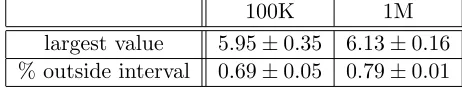
Empirically, one would have expected the use of bounded models to help a lot (in abso-lute terms), if learning just trace-norm constrained matrices (without clipping/bounding) leads to many predictions being outside the interval [1,5], in which we know the ratings lie. But indeed, this does not seem to be the case. Table 2 shows the prediction with largest magnitude, over all entries in the test set, as well as the percentage of predictions which fall outside the [1,5] interval. It is clearly evident that such out-of-interval predictions are relatively rare, and this explains why the bounding and clipping only leads to modest improvements.
100K 1M
largest value 5.95±0.35 6.13±0.16 % outside interval 0.69±0.05 0.79±0.01
Table 2: Out-of-Interval Values
We emphasize that our results should only be interpreted in the context of pure trace-norm regularization. There are many other approaches to matrix completion, and it is quite possible that using bounded models has more or less impact in the context of other approaches or for other application domains.
8. Follow-Up Work
While this work focuses on a stochastic setting, a closely related problem has been matrix completion in an online setting. In online learning (Cesa-Bianchi and Lugosi, 2006; Shalev-Shwartz, 2012), rather than having examples sampled from a stochastic process, the examples arrive in an online fashion and are arbitrary, possibly provided by an all-powerful adversary. The goal in this setting is to minimize regret, namely the difference between the learner’s loss and that of the best single hypothesis from some hypothesis class. In the context of matrix completion, this can be modeled as a sequential game where at each round a matrix entry is arbitrarily chosen, and the learner needs to predict its value. The actual entry value is then revealed, and the learner suffers some loss (such as the absolute difference between the prediction and actual value). In our case, the regret can be measured with respect to the class of matrices with bounded trace-norm. Note that this setting is generally harder than our stochastic setting, since the entry are chosen arbitrarily rather than in a stochastic manner, and it is known that in general, any online learning algorithm can be converted to a learning algorithm in a stochastic setting, with similar guarantees. Despite the difference between the settings, regret guarantees in the online learning setting are often strikingly similar to sample complexity guarantees in the stochastic learning setting.
The problem of online matrix completion with trace-norm bounded matrix has been dealt with in several recent works. Interestingly, the same insights provided in our work — the importance of entry boundedness or a transductive model — were crucial for attaining online learning algorithms. Consideringn×mmatrices with bounded trace-normtas well as bounded entries, Hazan et al. (2012) showed that one can efficiently obtain vanishing regret after O(t√n) rounds (assuming m ≤ n). Note that this parallels our sample complexity guarantees in a stochastic setting (assuming bounded entries), which imply learnability for sample size O(t√n). Alternatively, if one considers a transductive online setting (where each entry can be chosen only once), Cesa-Bianchi and Shamir (2011) showed that one can also efficiently obtain vanishing regret after O(t√n) rounds. In Rakhlin et al. (2012) this was shown to be possible for Lipschitz-continuous losses, even if the entries are not explicitly bounded — the transductive setting alone suffices to achieve results of this order.
Another recent related work is Shalev-Shwartz et al. (2011), which deals with a sup-posedly different problem: Approximately solving convex optimization problems over the (non-convex) domain of low-rank matrices. However, one of their results provides an alter-native justification of our O(t√n) sample complexity guarantee, for the case of bounded trace-norm matrices whose entries are clipped to a bounded range (Theorem 3). To sketch the argument, Shalev-Shwartz et al. (2011, Section 4) show that if we have |S| observed entries in our matrix, then for every matrixW with bounded trace-normkWktr, there exists a low-rank matrix ¯W, with rank O(kWk2
tr/|S|), which approximatesW arbitrarily well in terms of average loss over the observed entries. Since a matrix of rankr is parameterized by
O(rn) parameters, it follows that the generalization error of clipped r-rank matrices is ar-bitrarily small when|S| ≥Ω(˜ rn). This indirectly provides a generalization error bound for our original matrixW. Plugging inr=kWk2
tr/|S|, and noting that in our casekWktr =n, we get that learnability is possible for a sample of size|S| ≥Ω(˜ n3/2) = ˜Ω(t√n).
2012). An important motivation of these works is that they allow us to learn non-trivial classes of matrices, with a sample complexity of O(n) — smaller than earlier trivial re-sults for the trace-norm and the O(n3/2) results we obtain here (when the trace-norm is Θ(n)). Essentially, this is achieved by using classes of matrices which are less rich than trace-norm-bounded one, hence are statistically easier to learn.
9. Proofs of Upper Bounds
In our proofs, we usek · ksp to denote the spectral norm of matrices, which is well-known to be the dual of the trace-norm (see for instance Fazel et al., 2001).
Our proofs utilize the following two theorems, which bounds the expected spectral norm
k · ksp of random matrices.
Theorem 8 (Lata la, 2005) Let Z be a matrix composed of independent zero-mean en-tries. Then for some fixed constant C,E[kZksp]is at most
C
max
i
s X
j
E[Zi,j2 ] + max j
s X
i
E[Zi,j2 ] +4
s X
i,j
E[Zi,j4 ]
.
Theorem 9 (Seginer, 2000) Let A be an arbitrary m×n matrix, such that m, n > 1. Let Z denote a matrix composed of independent zero-mean entries, such that Zi,j = Ai,j
with probability 1/2 andZi,j =−Ai,j with probability1/2. Then for some fixed constantC,
E[kAksp] is at most
Cp4
log(min{m, n}) max
max i
s X
j
A2i,j,max j
s X
i
A2i,j
9.1 Proof of Theorem 2
We writeRS(`◦ W) as 1
|S|Eσ
sup
W∈W
X
i,j
Γi,j`(Wi,j, Xi,j)
, (7)
where Γ is a matrix whose (i, j)-th entry is defined as P
α:iα=i,jα=jσα. As discussed in
Section 3, a standard analysis will proceed to reduce this to
1
|S|Eσ
sup
W∈W
X
i,j
Γi,jWi,j
, (8)
bounded by a constant b`. Therefore, even if some Γi,j has a large value, it can only be multiplied by a factor as large as b`, andnot the trace-norm boundt. This observation is the key for our analysis.
Intuitively, instead of going directly from Equation (7) to Equation (8), we first de-compose Γ into two matrices Y and Z, where Y contains the “heavily-hit” entries, and
Z the “lightly-hit” entries, where the two types of entries are differentiated according to some threshold p. We perform a different type analysis for each matrix, and then tune p
appropriately to get the desired result.
More formally, given i, j, let hi,j be the number of times the sample S hits entry i, j, or more precisely hi,j =|{α :iα =i, jα =j}|. Let p >0 be an arbitrary parameter to be specified later, and define
Yi,j =
(
Γi,j hi,j > p 0 hi,j ≤p
Zi,j =
(
0 hi,j > p Γi,j hi,j ≤p.
(9)
Clearly, we have Γ =Y+Z. Thus, we can upper bound the Rademacher complexity by
1
|S|Eσ
sup
W∈W
X
i,j
Yi,j`(Wi,j, Xi,j)
+
1
|S|Eσ
sup
W∈W
X
i,j
Zi,j`(Wi,j, Xi,j)
. (10)
Since |`(Wi,j, Xi,j)| ≤b`, the first term can be upper bounded by
1
|S|Eσ
b`
X
i,j
|Yi,j|
=
b`
|S|Eσ[kYk1]. (11)
Using the Rademacher contraction principle,3 the second term in Equation (10) can be upper bounded by
l`
|S|Eσ
sup
W∈W
X
i,j
Zi,jWi,j
.
Applying H¨older’s inequality, and using the fact that the spectral normk · ksp is the dual to the trace norm k · ktr, we can upper bound the above by
l`
|S|EσWsup∈W
[kZkspkWktr] =
l`t
|S|Eσ[kZksp]. (12)
Combining this with Equation (11) and substituting into Equation (10), we get an upper bound of the form
b`
|S|Eσ[kYk1] + l`t
|S|Eσ[kZksp].
Using Lemma 10 and Lemma 11, which are given below, we can upper bound this by
b`
√ p +
2.2Cl`t
√
p(√m+√n)
|S| ,
wherepis the parameter used to defineY andZin Equation (9). Choosingp= |S|b`
2.2Cl`t(
√
m+√n),
we get the bound in the theorem.
Lemma 10 Let Y be a random matrix defined as in Equation (9). Then
E[kYk1]≤E
X
i,j:hi,j>p
p
hi,j
≤
|S| √
p
Proof E[kYk1] equals
E
X
i,j:hi,j>p
|Γi,j|
=E
E
X
i,j:hi,j>p
X
α:(iα,jα)=(i,j)
σα {hi,j}
The expression inside the absolute value is the sum of hi,j i.i.d. random variables, and it is easily seen that its expected absolute value is at most phi,j. Therefore, we can upper bound the above byE[Pi,j:hi,j>p
p
hi,j]. We can further upper bound it, in a manner which does not depend on the values ofhi,j, by
max
c∈{1,...,mn}h1,...,hc∈R:∀i hmaxi>p,Pci=1hi=|S|
c
X
i=1
p
hi.
Note that the constraints imply that
|S|= c
X
i=1 hi ≥
√ p c X i=1 p
hi,
soPc
i=1 √
hi can be at most|S|/
√
p as required.
Lemma 11 Let Z be a random matrix defined as in Equation (9). Then the expected spectral norm Eσ[kZksp]is at most
C max i s X
j:hi,j≤p
hi,j+ max j
s X
i:hi,j≤p
hi,j+4
s
3 X
i,j:hi,j≤p
h2i,j
,
where C is the universal constant which appears in the main theorem of Lata la (2005). Moreover, this quantity can be upper bounded by 2.2C√p(√m+√n)
Proof With hi,j held fixed, Z is a random matrix composed of independent entries. By using Theorem 8, we only need to analyzeE[Zi,j2 ] and E[Zi,j4 ]. For anyi, j, ifhi,j ≤p then
Zi,j is a sum ofhi,j i.i.d. variables taking values in{−1,+1}. Therefore, E[Zi,j2 ] =hi,j and
E[Zi,j4 ] ≤ 3h2i,j. Plugging into Theorem 8 yields the first part of the lemma. To get the second part, we can upper bound the right-hand side of the first part by
C√p
√
m+√n+√43mn
≤C√p
√
m+√n+p4
3/2(√m+√n)
9.2 Proof of Theorem 3
We can rewrite the definition ofRS(`◦ W) (see Equation 3) as
1
|S|Eσ
sup
W∈W
X
i,j
Γi,j`(Wi,j, Xi,j)
,
where Γ is a matrix defined as Γi,j =
P
α:iα=i,jα=jσα. Using the Rademacher contraction
principle (as in Meir and Zhang, 2003, Lemma 5), this is at most
l`
|S|Eσ
sup
W∈W
X
i,j
Γi,jWi,j
. (13)
Decomposing Γ = Y +Z as in Equation (9) according to a parameter p, we can upper bound the Rademacher complexity by
l`
|S|Eσ
sup
W∈W
X
i,j
Yi,jWi,j
+
l`
|S|Eσ
sup
W∈W
X
i,j
Zi,jWi,j
. (14)
By definition ofW,|Wi,j| ≤bφ, so the first term can be upper bounded by
l`
|S|Eσ
bφ X
i,j
|Yi,j|
=
l`bφ
|S|Eσ[kYk1]. (15)
The second term in Equation (14) equals
l`
|S|Eσ
sup
W:kWktr≤t
X
i,j
Zi,jφ(Wi,j)
≤
l`lφ
|S|Eσ
sup
W:kWktr≤t
X
i,j
Zi,jWi,j
,
again by the Rademacher contraction principle. Applying H¨older’s inequality, and using the fact that the spectral norm k · ksp is the dual to the trace norm k · ktr, we can upper bound the above by
l`lφ
|S|Eσ
"
sup W:kWktr≤t
kZkspkWktr
#
= l`lφt
|S| Eσ[kZksp].
Combining this with Equation (15) and substituting into Equation (14), we get an upper bound of the form
l`bφ
|S|Eσ[kYk1] + l`lφt
|S| Eσ[kZksp].
Using Lemma 10 and Lemma 11, we can upper bound this by
l`bφ
√ p +
2.2Cl`lφt
√
p(√m+√n)
|S| ,
wherepis the parameter used to defineY andZin Equation (9). Choosingp= |S|bφ
2.2Clφt(
√
m+√n),
9.3 Proof of Theorem 4
Before we begin, we will need the following technical result:
Lemma 12 The dual of the norm kWk= max{kWktr/t,kWk∞/b} equals kΓk∗ = min
Y+Z=ΓbkYk1+tkZksp, where kYk1=Pi,j|Yi,j|and kZksp is the spectral norm of Z.
It is possible to prove the lemma directly using duality of infimal convolution. However, for the sake of completeness we give below a self-contained proof.
Proof By definition of a dual norm, we have
kΓk∗= sup
W:kWk≤1
hΓ, Wi,
and our goal is to show that
sup W:kWk≤1
hΓ, Wi= min
Y+Z=ΓbkYk1+tkZksp.
First, we recall that the dual norm of kWktr is the spectral normkWksp, and the dual of
kWk∞ is the 1-normkWk1 =
P
i,j|Wi,j|. Now, for anyY, Z such thatY +Z = Γ, we have by H¨older’s inequality that
sup W:kWk≤1
hΓ, Wi= sup W:kWk≤1
hY, Wi+hZ, Wi
≤ sup W:kWk≤1
kYk1kWk∞+kZkspkWktr
≤bkYk1+tkZksp.
This holds for anyY, Z, and in particular
sup W:kWk≤1
hΓ, Wi ≤ min
Y+Z=ΓbkYk1+tkZksp. (16)
It remains to show the opposite direction, namely
sup W:kWk≤1
hΓ, Wi ≥ min
Y+Z=ΓbkYk1+tkZksp.
To show this, let W∗ be the matrix which maximizes the inner product above. We know that kW∗k ≤ 1, which means that either kW∗k∞ ≤ b, or kW∗ktr ≤ t. If kW∗k∞ ≤ b, it
follows that
sup W:kWk≤1
hΓ, Wi= sup W:kWk∞≤b
hΓ, Wi=bkΓk1≥ min
Y+Z=ΓbkYk1+tkZksp.
In the other case, if kW∗ktr ≤t, it follows that sup
W:kWk≤1
hΓ, Wi= sup W:kWktr≤t
hΓ, Wi=tkΓksp ≥ min
So in either case,
sup W:kWk≤1
hΓ, Wi ≥ min
Y+Z=ΓbkYk1+tkZksp.
Combining this with Equation (16), the result follows.
We now turn to the proof of Theorem 4 itself. Since `(Wi,j, Xi,j) is assumed to be
l`-Lipschitz, we can use the Rademacher contraction principle to upper bound RS(`◦ W) by
l`Eσ
sup
W∈W
1
|S| |S|
X
α=1
σαWiα,jα
=
l`
|S|Eσ
sup
W∈W
X
i,j
Γi,jWi,j
,
where Γ is a matrix defined as Γi,j =Pα:iα=i,jα=jσα.
Thinking of Γ, W as vectors, the equation above is the expected supremum of an inner product between Γ andW. By H¨older’s inequality, we can upper bound this by
l`
|S|Eσ
sup W∈W
kΓk∗kWk
(17)
for any normk · k and its dual normk · k∗. In particular, we will choose the normkWk=
max{kWktr/t,kWk∞/b}. Note that by definition of W, supW∈WkWk ≤ 1. Also, by
Lemma 12,
kΓk∗ = min
Y+Z=ΓbkYk1+tkZksp,
wherekYk1=Pi,j|Yi,j|, andkZksp is the spectral norm of Z . Thus, we can upper bound Equation (17) by
l`
|S|EΓ
min
Y+Z=ΓbkYk1+tkZksp
. (18)
Recall that Γ is random matrix, where each entry is the sum of Rademacher variables. Let
hi,j denote the number of variables ’hitting’ entry (i, j) — formally,hi,j =|{α: (iα =i, jα=
j}|. We can upper bound Equation (18) by replacing the optimal decomposition of Γ into
Y, Z by any fixed decomposition rule. In particular, for an arbitrary parameter p, we can decompose Γ intoY, Z as in Equation (9), and get an upper bound on Equation (18) of the form
l`
|S|(bEΓ[kYk1] +tEΓ[kZksp]). (19)
Bounds for the two expectations are provided in Lemma 10 and Lemma 11. Plugging them in, we get
bl`
√ p +
2.2l`Ct
√
p(√m+√n)
|S| .
Choosingp= 2.2Ct(b√|S|
9.4 Proof of Theorem 6
We writeRS(`◦ W) as 1
|S|Eσ
sup
W∈W
X
i,j
Γi,j`(Wi,j, Xi,j)
,
where Γ is a matrix with σi,j in its (i,j)-th entry, if (i, j) ∈ S, and 0 otherwise. By the Rademacher contraction property,4 we can upper bound this by
l`
|S|Eσ
sup
W∈W
X
i,j
Γi,jWi,j
.
By H¨older’s inequality, this is at most
l`
|S|Eσ
sup W∈W
kΓkspkWktr
= l`t
|S|Eσ[kΓksp]. (20)
The setting so far is rather similar to the one we had in the inductive setting (see the proof of any of the theorems in Section 4). But now, we need to bound just the expected spectral norm of Γ, which is guaranteed to have only a single Rademacher variable in each entry. By applying Theorem 8 on Equation (20), we get
RS(`◦ W)≤Cl`
t
√
M+√N +p4 |S| |S| .
SinceScan contain at mostmandnindices for any single row and column respectively, and
4
p
|S| ≤√4mn≤ 1 2(
√
m+√n), we can upper bound the above by 3Cl`t(
√
m+√n)/(2|S|). To get the other bound in the theorem, we apply Theorem 9 instead of Theorem 8 on Equation (20).
10. Discussion
In this paper, we analyzed the sample complexity of matrix completion with trace-norm regularization, obtaining the first non-trivial, distribution-free guarantees. Our results were based on either mild boundedness assumptions, or a switch from the standard inductive learning model to the transductive learning model. Moreover, we argue that such a trans-ductive model may be a better way to model matrix completion as performed in practice, as it seems more natural and leads to a substantial difference in terms of obtainable results. We also discussed the issue of learning with bounded models, and provided an empirical study which indicates that these lead to a modest improvement in performance, in line with our theoretical findings. We also show that our results are essentially tight, and discuss some recent work which relates to the results and insights provided here.
One interesting open question arises from our experiments in Section 7. In all our exper-iments, minimizing the squared loss over the training data (with trace-norm regularization)
resulted in matrices whose entries have reasonably small values, even when boundedness was not enforced. This is probably an important factor in explaining why explicitly enforcing boundedness resulted in only a modest performance improvement. However, if boundedness is not enforced, there is no a-priori reason why the resulting matrix shouldn’t have some very large values (up to the trace-norm constraint) in some of the test set entries. Thus, we may raise the following conjecture: If we minimize training loss over data, consisting of bounded entries, over trace-norm constrained matrices, then the resulting matrix will have bounded entries as well. If this conjecture holds, it means that enforcing boundedness will always lead to only a modest performance improvement.
Acknowledgements
We thank Nati Srebro and Ruslan Salakhutdinov for helpful discussions.
References
F. Bach. Consistency of trace-norm minimization. Journal of Machine Learning Research, 9:1019–1048, 2008.
P. Bartlett and S. Mendelson. Rademacher and Gaussian complexities: Risk bounds and structural results. Journal of Machine Learning Research, 3:463–482, 2003.
O. Bousquet Boucheron, S. and G. Lugosi. Theory of classification: A survey of some recent advances. ESAIM: Probability and Statistics, 9:323 – 375, 2005.
E. Cand`es and B. Recht. Exact matrix completion via convex optimization. Foundations of Computational Mathematics, 9, 2009.
E. Cand`es and T. Tao. The power of convex relaxation: Near-optimal matrix completion.
IEEE Trans. Inform. Theory, 56(5):2053–2080, 2009.
N. Cesa-Bianchi and G. Lugosi. Prediction, Learning, and Games. Cambridge University Press, 2006.
N. Cesa-Bianchi and O. Shamir. Efficient online learning via randomized rounding. In
NIPS, 2011.
Ran El-Yaniv and Dmitry Pechyoni. Transductive rademacher complexity and its applica-tions. Journal of AI Research, 35:193–234, 2009.
M. Fazel, H. Hindi, and S. Boyd. A rank minimization heuristic with application to minimum order system approximation. In American Control Conference, 2001. Proceedings of the 2001, volume 6, pages 4734–4739. IEEE, 2001.
R. Foygel, R. Salakhutdinov, O. Shamir, and N. Srebro. Learning with the weighted trace-norm under arbitrary sampling distributions. In NIPS, 2011.
E. Hazan, S. Kale, and S. Shalev-Shwartz. Near-optimal algorithms for online matrix prediction. InCOLT, 2012.
R. Horn and C. Johnson. Matrix Analysis. Cambridge University Press, 1985.
M. Jaggi and M. Sulovsk´y. A simple algorithm for nuclear norm regularized problems. In
ICML, 2010.
L. Kozma, A. Ilin, and T. Raiko. Binary principal component analysis in the netflix collab-orative filtering task. In IEEE MLSP Workshop, 2009.
R. Lata la. Some estimates of norms of random matrices. Proceedings of the AMS, 133(5): 1273–1282, 2005.
J. Lee, B. Recht, R. Salakhutdinov, N. Srebro, and J. Tropp. Practical large-scale optimiza-tion for max-norm regularizaoptimiza-tion. In NIPS, 2010.
H. Ma, H. Yang, M. Lyu, and I. King. Sorec: social recommendation using probabilistic matrix factorization. InCIKM, 2008.
R. Meir and T. Zhang. Generalization error bounds for bayesian mixture algorithms.Journal of Machine Learning Research, 4:839–860, 2003.
S. Negahban and M. Wainwright. Restricted strong convexity and weighted matrix com-pletion: Optimal bounds with noise. arXiv:1009.2118, 2010.
M. Piotte and M. Chabbert. The pragmatic theory solution to the netflix grand prize. Available at http://www.netflixprize.com/assets/GrandPrize2009_BPC_ PragmaticTheory.pdf, 2009.
A. Rakhlin, O. Shamir, and K. Sridharan. Relax and randomize : From value to algorithms. In NIPS, 2012.
R. Salakhutdinov and A. Mnih. Probabilistic matrix factorization. In NIPS, 2007.
R. Salakhutdinov and N. Srebro. Collaborative filtering in a non-uniform world: Learning with the weighted trace norm. In NIPS, 2010.
Y. Seginer. The expected norm of random matrices. Combinatorics, Probability & Com-puting, 9(2):149–166, 2000.
S. Shalev-Shwartz. Online learning and online convex optimization.Foundations and Trends in Machine Learning, 4(2):107–194, 2012.
S. Shalev-Shwartz, A. Gonen, and O. Shamir. Large-scale convex minimization with a low-rank constraint. InICML, 2011.
O. Shamir and S. Shalev-Shwartz. Collaborative filtering with the trace norm: Learning, bounding, and transducing. In COLT, 2011.
N. Srebro and A. Shraibman. Rank, trace-norm and max-norm. InCOLT, 2005.
N. Srebro, J. Rennie, and T. Jaakkola. Maximum-margin matrix factorization. In NIPS, 2004.
K. Toh and S. Yun. An accelerated proximal gradient algorithm for nuclear norm regularized least squares problems. Optimization Online, 2009.