A Monte Carlo simulation study comparing linear regression, beta regression, variable-dispersion beta regression and fractional logit regression at recovering average difference measures in a two sample design

(1)

R E S E A R C H A R T I C L E

Open Access

A Monte Carlo simulation study comparing linear

regression, beta regression, variable-dispersion

beta regression and fractional logit regression at

recovering average difference measures in a two

sample design

Christopher Meaney

*

and Rahim Moineddin

Abstract

Background:In biomedical research, response variables are often encountered which have bounded support on the open unit interval - (0,1). Traditionally, researchers have attempted to estimate covariate effects on these types of response data using linear regression. Alternative modelling strategies may include: beta regression, variable-dispersion beta regression, and fractional logit regression models. This study employs a Monte Carlo simulation design to compare the statistical properties of the linear regression model to that of the more novel beta regression, variable-dispersion beta regression, and fractional logit regression models.

Methods:In the Monte Carlo experiment we assume a simple two sample design. We assume observations are realizations of independent draws from their respective probability models. The randomly simulated draws from the various probability models are chosen to emulate average proportion/percentage/rate differences of pre-specified magnitudes. Following simulation of the experimental data we estimate average proportion/percentage/rate differences. We compare the estimators in terms of bias, variance, type-1 error and power. Estimates of Monte Carlo error associated with these quantities are provided.

Results:If response data are beta distributed with constant dispersion parameters across the two samples, then all models are unbiased and have reasonable type-1 error rates and power profiles. If the response data in the two samples have different dispersion parameters, then the simple beta regression model is biased. When the sample size is small (N0= N1= 25) linear regression has superior type-1 error rates compared to the other models. Small

sample type-1 error rates can be improved in beta regression models using bias correction/reduction methods. In the power experiments, variable-dispersion beta regression and fractional logit regression models have slightly elevated power compared to linear regression models. Similar results were observed if the response data are generated from a discrete multinomial distribution with support on (0,1).

Conclusions:The linear regression model, the variable-dispersion beta regression model and the fractional logit regression model all perform well across the simulation experiments under consideration. When employing beta regression to estimate covariate effects on (0,1) response data, researchers should ensure their dispersion sub-model is properly specified, else inferential errors could arise.

Keywords:Regression modelling, Linear regression, Beta regression, Variable-dispersion beta regression, Fractional Logit regression, Beta distribution, Multinomial distribution, Monte Carlo simulation

* Correspondence:[email protected]

Department of Family and Community Medicine, University of Toronto, 500 University Avenue, Toronto M5G1V7, ON, Canada

© 2014 Meaney and Moineddin; licensee BioMed Central Ltd. This is an open access article distributed under the terms of the Creative Commons Attribution License (http://creativecommons.org/licenses/by/2.0), which permits unrestricted use, distribution, and reproduction in any medium, provided the original work is properly cited.

(2)

Background

In biomedical research it is common to encounter re-sponse variables which have support on the interval (0,1). These types of response variables may arise in the form of proportions/percentages, or certain types of fractions and rates. The traditional approach to analyz-ing these types of response data–across virtually all sci-entific disciplines - is via linear regression. If desired, the response variable can be transformed prior to estimation of the linear regression parameters. This transformed linear model may improve diagnostic performance; how-ever, this may render interpretation of estimated regression parameters challenging. Alternatively, the beta distribution allows specification of a probability model for continuous random variables with support over the interval (0,1). For many years statisticians have exploited the flexibility of the beta distribution in theoretical modelling exercises; how-ever, its use in applied research settings has not garnered equal attention. Johnson et al. [1] cite numerous instances where the beta distribution has been used in theory/prac-tice and champion increased use of the beta distribution in applied research settings. Gupta et al. [2] also cite numer-ous applications where the beta distribution provides a use-ful probability generating model for continuous data with support on the interval (0,1). However, neither of these ex-tensive resources on the beta distribution cites a regression modelling framework for estimating covariate effects on beta distributed response variables. Recent developments by Paulino [3], Ferrari and Cribrari-Neto [4], Smithson and Verkuilen [5] and others have resulted in a more general purpose beta regression machinery. The variable-dispersion beta regression model [5] will be used extensively in our simulation experiments, as it is particularly useful for mod-elling covariate effects on response variables which are as-sumed to follow a beta distribution. The beta regression model extends on ideas of generalized linear models [6] both in terms of their specification and estimation. Use of the beta regression model has been increasing in recent years. In slides from an unpublished presentation given by Ferrari [7], the author suggests over 100 instances where beta regression has been used in theoretical and applied re-search settings. Some application areas include: medicine, veterinary science, pharmacology, odontology, hydrobiol-ogy, nutritional science, forest science, waste management, education, political science, economics and finance. Clearly, embedding the beta distribution within a more general re-gression modelling framework has enhanced its uptake in applied research settings. A final model which we consider for estimating the average proportion/percentage/rate dif-ference in our two-sample model is the fractional logit re-gression model. The fractional logit model is a popular model for fractional response variables in econometrics and was proposed (independently) by Papke and Wooldridge [8] and by Cox [9]. The fractional logit model is similar to

generalized linear regression models [6]; however, it does not make any fully parametric assumptions regarding the distributional form for the response variable. Rather the fractional logit model only specifies a parametric form for the conditional mean and conditional variance of the re-sponse. The form of the conditional mean and variance functions are chosen to ensure admissible predictions/fit-ted-values from such models. In this case, the model speci-fication is chosen to ensure predictions/fitted values from the fractional logit model fall in the interval (0,1). The estimator proposed by Papke and Wooldridge [8] is the one we pursue in this manuscript as they specify forms for robust variance estimators which have more desirable coverage/power properties than the more traditional quasi-likelihood models proposed by Cox [9].

Given the recent popularity of the beta regression model, especially in biomedical research, we thought it prudent to compare linear regression, beta regression, variable-dispersion beta regression and fractional logit regression models for estimating covariate effects on a response variable which lives on the interval (0,1). To accomplish this goal we conducted a Monte Carlo simu-lation experiment where we generated response variables following different (parametric) probability generating models. First, we considered simulating response data from the continuous beta distribution with support on (0,1). This experiment allows us to compare models when we know the beta regression model is properly specified given the response data. Specifically, we can in-vestigate efficiency gains which may be observed from specifying an appropriate statistical model to observed response data. Additionally, we simulate response data from the discrete multinomial distribution with prob-ability mass observed only on a finite number of points in (0,1). This experiment allows us to investigate model performance when response data is non-continuous. In this case, all models are incorrectly specified given the response data. This experiment allows us to investigate whether estimated regression models are robust to non-continuous response data. In all scenarios, we fit linear regression, beta regression, variable-dispersion beta re-gression, and fractional logit regression models to these randomly generated response data and compared the finite sample statistical properties of the respective esti-mators. We are particularly interested in the ability of each estimator to recover the average proportion/per-centage/rate differences from a simple two sample de-sign. In terms of statistical properties we will compare the respective estimators in terms of: bias, variance, type-1 error and power. Understanding the performance of these models on simulated datasets (where population parameters are known) is important for applied re-searchers who must discern whether to estimate covari-ate effects on (0,1) response data using the traditional

Meaney and MoineddinBMC Medical Research Methodology2014,14:14 Page 2 of 22

(3)

linear regression model or more novel regression models, such as beta regression, variable-dispersion beta regression and fractional logit regression models.

Methods

Statistical methods

The linear regression model

The linear regression model is a workhorse of applied statisticians. It is used to model the effect of continuous/ categorical covariates on a scalar response (assumed to be generated according to a Gaussian probability model). Thorough introductions to the linear regression model are given in Weisberg [10], McCullagh and Nelder [6], and White [11].

In this study we consider a simple two sample prob-lem, re-cast under a regression framework, such that our response variable is modelled as a function of a single intercept parameter and a single slope parameter. The linear model and its conditional mean function look as follows:

Yi¼β0þβ1Xi1þεi E Yð jiXiÞ ¼β0þβ1Xi1

The notation above suggests that we observe a vector of response variables, Y1…Yn. Further, we have informa-tion on a single binary covariate, Xi∈{0,1}, again for i = 1…n. The regression coefficientsβ0and β1are estimated from the data. Estimation and inferential procedures are justified given that the following assumptions are satis-fied [11]:

1. The model is properly specified

2. X is a non-stochastic and finite dimensional (n by p) matrix with n≥p

3. (XTX) is non-singular and hence invertible 4. E(εi) = 0∀(i = 1…n)

5. εi~ Normal(0,σ2)∀(i = 1…n)

In our experiment, we are interested in the ability of the linear regression estimator to recover the average proportion/percentage/rate difference given our simple two sample design. Taking linear combinations of the es-timated model parameters we arrive at the following estimator:

Δ¼E Yi Xi1¼1Þ−E YiXi1¼0Þ ¼β1

Therefore a test ofΔ= 0 is equivalent to a test ofβ1= 0. In this simulation we carry out such a test using a Wald statistic, W, which follows an asymptotic standard normal distribution. We reject the null hypothesis in in-stances where |W| > 1.96 (corresponding to an α= 5% significance threshold).

The beta regression model (and some extensions)

The beta regression model was proposed by Paulino [3], Ferrari and Cribrari-Neto [4], and Smithson and Verkuilen [5] for modelling covariate effects on a con-tinuous response variable which assumes support on the interval (0,1).

The beta distribution is thoroughly described in Johnson et al. [1] and Gupta [2]. The beta density is a very flexible density, assuming support on the interval (0,1). The most common parameterization of the beta density is in terms of its two shape parameters {p,q}:

f yð ;p;qÞ ¼ΓðpþqÞ

Γð Þp Γð Þq yp−1ð1−yÞ

q−1

In the parameterization given above we assume p > 0, q > 0, y ∈(0,1) and use Γ(·) to denote the gamma func-tion (a generalizafunc-tion of the factorial funcfunc-tion to non-integer arguments). The density assumes probability mass on the interval (0,1) and is zero elsewhere. Further, under this parameterization we define the mean and variance of the random variable, Y, as follows:

E Yð Þ ¼_pp þq

VAR Yð Þ ¼ pq

pþq

ð Þ2 _p_þ_q_þ 1

ð Þ

Above E(·) and VAR(·) denote the expectation and variance operators, with respect to the given beta distri-bution. In regression modelling, it is more common to parameterize the density in terms of a mean (μ) and dis-persion parameter (φ) instead of two shape parameters, {p,q}. In this parameterization we have the following relationships:

μ¼_pp þq

φ¼pþq

This implies:p=μφandq= (1–μ)φ.

Given the above relationships we can derive the mean and the variance of the beta density in terms of a mean and dispersion parameter as follows:

E Yð Þ ¼μ

VAR Yð Þ ¼Vð Þμ

1þφ¼

μð1−μÞ 1þφ

Given a fixed value for the mean, the larger the value ofφthe smaller the variance of the response variable, Y (and vice-versa). Under this new parameterization, in terms of a mean and dispersion parameter, the density of Y looks as follows:

(4)

f yð ;μ;φÞ ¼ Γ φð Þ

Γ μφð ÞΓðð1−μÞφÞy

μφ−1_ð₁₋_y_Þð1−μÞφ−1

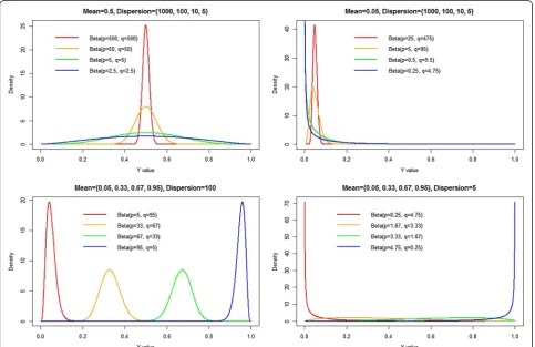
In Figure 1, we graphically represent some of the forms the beta density can take on for different values of {p,q}, or alternatively, {μ,φ}.

The beta regression model, and the variable-dispersion extensions which we will discuss in this study are being increasingly utilized to model covariate effects on re-sponse variables observed on the interval (0,1). The beta regression model is an obvious choice for modelling re-sponse data which follow a beta distribution. Consider the scenario where we observe response data Y1…Yn on the interval (0,1). The beta regression model assumes that the mean of these random variables, can be repre-sented in the following form:

gð Þ ¼μi ηi¼β0þβ1Xi1

Our link function g(·) can be any function which is strictly monotone, twice differentiable, and maps the re-sponse variable observed on the interval (0,1) to the real line. The most commonly used link function in beta

regression is the logit link. Alternative link functions in-clude: the probit, the complementary log-log, the log-log and the Cauchy link. In general, any inverse cumulative distribution function will be an appropriate link function in a beta regression framework as they act to map the interval (0,1) to the real line.

The components of the basic beta regression model can be summarized as:

1. A response variable from a beta distribution 2. A linear predictor,ηi

3. A suitable link function, such that:E(Yi|Xi) =g(μi) =ηi

Given the above components, the log-likelihood of the beta regression model can be written as follows:

LLðμi;φÞ ¼logΓ φð Þ−logΓ μð iφÞ−log 1ðð −μiÞφÞ þðμiφ−1Þlogð Þyi

þfð1−μ_iÞφ−1glog 1ð −y_iÞ

The log-likelihood function can be maximized numer-ically as described in Ferrari and Cribrari-Neto [4]. The

Figure 1Various forms of the beta density for varying shape parameters {p,q}.Top left panel: We fix the mean equal to 0.5 and plot the

resulting beta densities for varying dispersion parameters. Top right panel: We fix the mean equal to 0.05 and plot the resulting beta densities for varying dispersion parameters. Bottom left panel: We fix the dispersion parameter equal to 100 and plot the resulting beta densities for varying mean parameters. Bottom right panel: We fix the dispersion parameter equal to 5 and plot the resulting beta densities for varying mean parameters.

(5)

mean and dispersion parameter estimates are known to be biased, especially in small samples. Kosmidis and Firth [12] discuss the issue of finite sample bias in beta regression. The authors propose a general purpose algo-rithm for producing bias-reduced and bias-corrected parameter estimates via adjustments to the score function. In our simulation experiment we estimate parameters from the beta regression model via standard maximum likeli-hood (ML) methods, as well as the bias-reduced (BR) and bias-corrected (BC) methods. In our simulation experi-ments we employ the simple ML estimators; however, we note that BC/BR methods may improve type-1 error rates in small sample situations.

The beta regression model proposed above assumes that the dispersion parameter is constant for all individ-uals under consideration. In many biomedical applica-tions this may be an unrealistic assumption (especially if one expects a non-zero mean difference across categor-ical groups). As its name implies, the variable-dispersion beta regression model [5] allows the value of the disper-sion parameter to vary across individuals. Further, the value of the dispersion parameter can actually be mod-elled as a function of covariates. The variable-dispersion beta regression model is a type of double-index regres-sion model [13], as it contains two regresregres-sion equations, one modelling the mean as a function of covariates and the other modelling the dispersion as a function of covariates.

Again, we consider the scenario where we observe re-sponse data Y1…Yn on the interval (0,1). The variable-dispersion beta regression model assumes that the mean and dispersion of these random variables can be repre-sented in the following form:

gð Þ ¼μi ηi¼β0þβ1Xi1 hð Þ ¼φi ζi¼γ0þγ1Xi1

Once again, we assume that both g(·) and h(·) are strictly monotonic, twice differentiable functions which act to map the mean, μi, and the dispersion, φi, to the real line. Once again, suitable choices of g(·) include the following link functions: logit, probit, complementary log-log, log-log, Cauchy or any other inverse cumulative distribution function. The link function for h(·) is typic-ally chosen to be the log link. The identity link can also be used; however, it has the undesirable property of pos-sibly suggesting non-positive values ofφi.

The log-likelihood function for the variable-dispersion beta regression model can be numerically maximized and is subject to similar finite sample biases as the basic beta regression model. Below, we illustrate the log-likelihood function for this model:

LLðμi;φÞ ¼logΓ φð Þi −logΓ μð iφiÞ−log 1ðð −μiÞφiÞ þðμiφi−1Þlogð Þyi

þfð1−μ_iÞφ_i−1glog 1ð −y_iÞ

In the case of both the beta regression model and the variable-dispersion (double-index) beta regression models, estimates of mean and dispersion parameters {β,γ} are achieved by numerically solving the likelihood equations given above. The resulting parameter esti-mates are asymptotically normally distributed and take the following form:

β̂

γ̂ eMVN β_γ ;C−1

Further,

C−1_¼_C−1_ð_β_;_γ_{Þ ¼} Cββ Cβγ Cγβ _Cγγ

For our purposes it suffices to realize that the estima-tors of the mean and dispersion parameters are consist-ent estimators of their target parameters and are distributed according to a multivariate normal distribu-tion, with variance-covariance matrix C-1. Detailed deri-vations of these formulas (particularly pertaining to the forms of the C-1 matrix) are given in Ferrari and Cribrari-Neto [4].

Again, we are interested in the ability of the (variable-dispersion) beta regression estimator to recover the aver-age proportion/percentaver-age/rate difference given our two sample design. In all of our simulation experiments we assume a logit link for the mean function. The (default) identity link is used in the beta regression modelling context and the log link is used in the variable-dispersion beta regression context. In all scenarios, our target of inference is the average proportion/percentage/ rate difference and we view the terms in the dispersion sub-model as a nuisance. A point estimator of the pro-portion/percentage/rate difference from the beta regres-sion model is:

Δ¼log 1

1þ exp −β₀−β₁Xi1

!

−log 1

1þ exp−β₀

!

We use the delta method to estimate the variance and standard error of this estimator, respectively. We con-struct a Wald style test of the null hypothesis thatΔ= 0. The Wald statistic, W, is computed as the ratio of the difference in proportion/percentage/rates over the esti-mated standard error. The test statistic is presumed to follow an asymptotic standard normal distribution. Again, we use a 5% critical threshold for rejecting the null hypothesis (this corresponds to rejection of H0if |W| > 1.96)

(6)

The fractional logit regression model

The final methodology we consider for estimating aver-age proportion/percentaver-age/rate differences in our two-sample design is the fractional logit regression model [8,9]. The fractional logit regression model is most com-monly encountered in the econometrics literature and has been demonstrated as being an effective means for estimating covariate effects on a response variable which lives on (0,1). Hence we consider it in this manuscript– as a result, introducing health services researchers to yet another plausible strategy for modelling proportions/ percentages/fractions/rates.

The fractional logit regression model is considered a quasi-parametric regression model. In other words, the fractional logit regression model does not make any parametric assumption regarding the distribution of the response variable being modelled; rather, it makes as-sumptions regarding only the first two conditional mo-ments of the response variable – the conditional mean and the conditional variance. The choice of the condi-tional mean and condicondi-tional variance function are typic-ally made to ensure that predictions/fitted-values from the specified model are admissible. In our case, this im-plies that the predictions/fitted-values fall in the interval (0,1).

As mentioned above, quasi-likelihood models typically only make assumptions regarding the first two condi-tional moments of the response variable [6, 9]. The con-ditional variance is assumed to be a known function of the mean (up to a scale parameter) and the conditional mean function therein is assumed to be a function of unknown model parameters:

V Yð jiXiÞ ¼σ2ν μð Þi

E Yð jiXiÞ ¼gð Þ ¼μi β0þβ1Xi1þ…þβpXip

In the first Equation V(·) denotes the variance oper-ator,σ2is a scale parameter which is estimated from ob-served data. ν(·) is a known variance function, and μiis the mean function. In the second Equation E(·) denotes the variance operator, g(·) is a known link function and

βj represent the unknown mean function parameters which must be estimated from the data. Yiand Xi rep-resent the response variable and observed covariates, respectively.

In describing the fractional logit model we adopt the terminology of Papke and Wooldridge [8]. Our chief as-sumption relates to the specification of the conditional mean function, namely:

E Yð Þ ¼i hð Þμi

Generally, h(·) is a known function which maps our real valued linear predictor into the interval (0,1). Again,

their exist many plausible function which could accom-plish this goal, in this manuscript we choose h(·) to be the logistic function and arrive at the fractional logit model. That is:

hð Þ ¼μi

expð Þμi

1þexpð Þμi ¼

1 1þexpð−μiÞ

Further, the conditional variance of the response variable is assumed to be:

V Yð jixiÞ ¼σ2ðhð Þμi ð1−hð Þμi ÞÞ

Papke and Wooldridge [8] argue that this conditional variance assumption is too restrictive for modelling response data with support over (0,1). Therefore, in their manuscript they offer two alternative strategies: first, using robust/sandwich estimators of the variance-covariance matrix and second, adjusting the estimated variance-covariance matrix by the Pearson scale adjust-ment factor. We considered both approaches; however, noted little difference in performance between the two estimators of the variance-covariance matrix. Hence, we report on only the fractional logit model with sandwich/ robust variance-covariance matrix.

Parameter estimation under the fractional logit model proceeds by maximizing the following Bernoulli quasi-likelihood function:

LL¼y_ilog hð ð Þμi Þ þð1−yiÞ log hð ð Þμi Þ

Monte Carlo simulation design

The goal of this simulation experiment is to compare the properties of the linear regression model, the beta regression model, the variable-dispersion beta regression model and the fractional logit regression model at recov-ering estimates of average proportion/percentage/rate differences from a simple two sample design. In all ex-periments we simulate data from parametric probability generating models such that the observed response data is on the interval (0,1). Subsequently, we estimate covari-ate effects on the response variable using one of four re-gression models: the linear rere-gression model, the beta regression model, the (double-index) variable-dispersion beta regression model and the fractional logit regression model. Given estimates of average proportion/percent-age/rate differences from the respective models, we compare statistical properties of the respective estima-tors, such as: bias, variance, type-1 error and power [14,15]. We investigate finite sample performance of each of the estimators by varying the sample size within each unique simulation experiment. In all scenarios, the sample size in group 1 is set equal to the sample size in group 2. Group specific sample sizes under consider-ation in this simulconsider-ation are: 25, 100, 250, and 750. The

(7)

total sample size for a given simulation experiment is double the group-specific sample size (as this experi-ment assumes a 2-sample design). In each instance we consider 20,000 replications of each experiment. We choose 20,000 replicate simulations such that coverage in the type-1 error experiments is based off of approxi-mately 1000 rejections of a true null hypothesis. We present mean estimates of bias, variance, type-1 error and power averaged across the 20,000 replicate simula-tions. Further we present Monte Carlo error estimates of bias, variance and power. Detailed derivations of Monte Carlo error are described in White [16]. The “seeds” which govern the pseudo-randomness of the various Monte Carlo experiments are given in the attached R/ SAS codes.

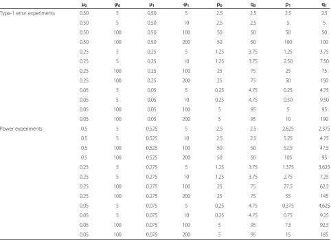
The first parametric probability model which we con-sider for generating response data on the interval (0,1) is the beta distribution. Table 1 describes the parameter values used to generate randomly simulated beta re-sponse variables. The rere-sponse variables are generated

such that certain mean and dispersion properties are achieved. For example, mean differences of zero are used to assess the type-1 error rates of respective estimators (for both fixed and varying dispersion). Further, non-zero mean differences are used to assess power (again for both fixed and varying dispersion). In this experi-ment response data are generated as independent draws from the respective beta distributions. That is, observa-tions within and between the two samples are independ-ently distributed. Within the type-1 error and power experiment frameworks, respectively, we have 3 sub-experiments: the first set of experiments consider the scenario where the central tendency of the simulated re-sponse distribution is near the center of the support (0.5); the second set of experiments considers the effect of shifting the central tendency to the right such that it is centered near 0.25; and finally, the last experiment considers the effect of shifting the central tendency to the boundary of the support, near 0.05. As sub-scenarios we vary the shape of the beta distribution when data are

Table 1 Description of 24 simulation experiments where the response variable is distributed according a beta distribution with the following mean and dispersion parameters in each respective group (or alternatively

parameterized in terms of its two shape parameters–p and q–in each group)

μ0 φ0 μ1 φ1 p0 q0 p1 q1

Type-1 error experiments 0.50 5 0.50 5 2.5 2.5 2.5 2.5

0.50 5 0.50 10 2.5 2.5 5 5

0.50 100 0.50 100 50 50 50 50

0.50 100 0.50 200 50 50 100 100

0.25 5 0.25 5 1.25 3.75 1.25 3.75

0.25 5 0.25 10 1.25 3.75 2.50 7.50

0.25 100 0.25 100 25 75 25 75

0.25 100 0.25 200 25 75 50 150

0.05 5 0.05 5 0.25 4.75 0.25 4.75

0.05 5 0.05 10 0.25 4.75 0.50 9.50

0.05 100 0.05 100 5 95 5 95

0.05 100 0.05 200 5 95 10 190

Power experiments 0.5 5 0.525 5 2.5 2.5 2.625 2.375

0.5 5 0.525 10 2.5 2.5 5.25 4.75

0.5 100 0.525 100 50 50 52.5 47.5

0.5 100 0.525 200 50 50 105 95

0.25 5 0.275 5 1.25 3.75 1.375 3.625

0.25 5 0.275 10 1.25 3.75 2.75 7.25

0.25 100 0.275 100 25 75 27.5 62.5

0.25 100 0.275 200 25 75 55 145

0.05 5 0.075 5 0.25 4.75 0.375 4.625

0.05 5 0.075 10 0.25 4.75 0.75 9.25

0.05 100 0.075 100 5 95 7.5 92.5

0.05 100 0.075 200 5 95 15 185

(8)

simulated from the center, right-center and far-right of the support, considering scenarios where the simulated data are symmetric and other scenarios where the simu-lated data is highly skewed. As the data are beta distrib-uted we expect the beta regression models to perform well in all scenarios; however, we anticipate that the lin-ear model will perform well when data are symmetric and unimodal. That is, we expect the linear model to perform well as the shape/rate parameters both become large and as the ratio of the shape/rate parameters ap-proach 1 (resulting in a symmetric and unimodal beta distribution – which converges to that of a normal distribution).

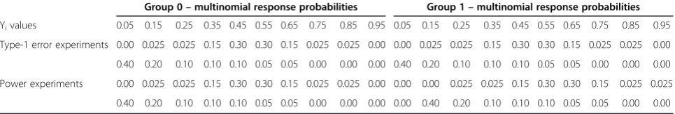
The next parametric probability model under consid-eration is the discrete multinomial model which takes probability mass only on a finite number of points on the interval (0,1). More specifically, we assume our re-sponse variable Yican take on the following values:

Yi∈f0:05;0:15;0:25;0:35;0:45;0:55;0:65;0:75;0:85;0:95g

That said, we do not assume the probability of assum-ing these values is necessarily uniform. Rather, we assign a vector of probabilities to these points, corresponding to the relative likelihood that the response variable as-sumes that particular value. Table 2 describes the par-ticular probability vectors used to generate response variables for each group in our two sample design. Once again, we vary the expected value of the response to as-sess differences in type-1 error rates and power across our linear regression, beta regression, (double-index) variable-dispersion beta regression and fractional logit regression models. Again, in this experiment response data are generated as independent draws from the re-spective multinomial distributions. That is, observations within and between the two samples are independently distributed.

Statistical software

This simulation experiment was conducted using R version 3.02 [17] and results were also verified using SAS 9.3 [18].

Simulation of the beta and multinomial response vari-ables were carried out using the rbeta() and rmultinom() functions, respectively. Linear regression modelling was performed using the lm() function. Beta regression was performed using the betareg() function in the betareg li-brary [13]. Fractional logit regression models were esti-mated using the glm() function and the sandwich() function [19]. Standard errors for the proportion/per-centage/rate differences from beta regression and frac-tional logit regression models were calculated using the deltamethod() function in the msm library [20].

SAS PROC NLMIXED was used to specify the linear re-gression model, beta rere-gression model, variable-dispersion beta-regression model and fraction logit regression model likelihood equations, respectively, and model parameters were estimated via likelihood methods.

All R and SAS code used to conduct this simulation can be obtained by contacting the corresponding author.

Results

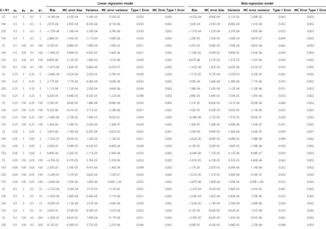
Detailed results of the Monte Carlo simulation study are given in Tables 3, 4, 5 and 6. Tables 3 and 4 describe the type-1 error and power experiments, respectively, given response data simulated according to independent draws from various parameterizations of the beta distribution. Tables 5 and 6 describe the type-1 error and power ex-periments, respectively, given response data simulated according to independent draws from various parame-terizations of the multinomial distribution.

Table 3 describes the results of the type-1 error experi-ment (Δ= 0) given response data distributed according to independent draws from a beta distribution. The top half of Table 3 illustrates results when the dispersion parameter is equal across groups; whereas, the bottom half of Table 3 illustrates results when the dispersion parameter varies as a function of group membership. As probability mass moves away from the center of the support (i.e. 0.5) and towards the boundary of the sup-port (0 or 1) we observe that the beta regression model provides biased estimates of the average proportion/per-centage/rate difference between the two samples when the dispersion parameters vary as a function of group

Table 2 Description of 4 simulation experiments where the response variable is distributed according to a discrete multinomial distribution on the points {0.05, 0.15, 0.25, 0.35, 0.45, 0.55, 0.65, 0.75, 0.85, 0.95} with corresponding probabilities of occurrence listed in the table for each of the two groups under consideration

Group 0–multinomial response probabilities Group 1–multinomial response probabilities

Yivalues 0.05 0.15 0.25 0.35 0.45 0.55 0.65 0.75 0.85 0.95 0.05 0.15 0.25 0.35 0.45 0.55 0.65 0.75 0.85 0.95

Type-1 error experiments 0.00 0.025 0.025 0.15 0.30 0.30 0.15 0.025 0.025 0.00 0.00 0.025 0.025 0.15 0.30 0.30 0.15 0.025 0.025 0.00 0.40 0.20 0.10 0.10 0.10 0.05 0.05 0.00 0.00 0.00 0.40 0.20 0.10 0.10 0.10 0.05 0.05 0.00 0.00 0.00 Power experiments 0.00 0.025 0.025 0.15 0.30 0.30 0.15 0.025 0.025 0.00 0.00 0.00 0.025 0.025 0.15 0.30 0.30 0.15 0.025 0.025 0.40 0.20 0.10 0.10 0.10 0.05 0.05 0.00 0.00 0.00 0.00 0.40 0.20 0.10 0.10 0.10 0.05 0.05 0.00 0.00

(9)

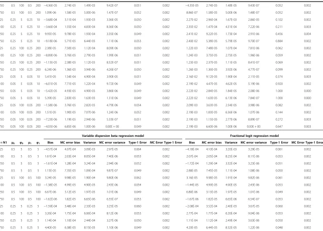
Table 3 Mean estimates from 20000 replicate simulations of bias (MC error of bias), variance (MC error of variance) and type-1 error (MC error type-1 error), from the fitted linear, beta, variable-dispersion beta and fractional logit regression models estimated on the beta distributed response data (Type 1 error experiments)

Linear regression model Beta regression model

N0 = N1 μ0 φ0 μ1 φ1 Bias MC error bias Variance MC error variance Type-1 Error MC Error Type-1 Error Bias MC error bias Variance MC error variance Type-1 Error MC Error Type-1 Error

25 0.5 5 0.5 5 −4.18E-04 4.10E-04 3.34E-03 3.35E-05 0.050 0.002 −4.52E-04 4.06E-04 3.11E-03 2.99E-05 0.063 0.002

100 0.5 5 0.5 5 2.07E-04 2.05E-04 8.33E-04 8.15E-06 0.050 0.002 1.65E-04 2.03E-04 8.06E-04 7.41E-06 0.052 0.002

250 0.5 5 0.5 5 −1.72E-04 1.29E-04 3.33E-04 3.24E-06 0.050 0.002 −1.57E-04 1.27E-04 3.25E-04 2.95E-06 0.052 0.002

750 0.5 5 0.5 5 2.88E-05 7.45E-05 1.11E-04 1.08E-06 0.050 0.002 1.20E-05 7.35E-05 1.09E-04 9.87E-07 0.049 0.002

25 0.5 100 0.5 100 3.16E-05 9.98E-05 1.98E-04 1.00E-05 0.051 0.002 3.25E-05 9.98E-05 1.90E-04 9.81E-06 0.062 0.002

100 0.5 100 0.5 100 −1.44E-05 4.99E-05 4.95E-05 2.44E-06 0.051 0.002 −1.38E-05 4.99E-05 4.90E-05 2.43E-06 0.054 0.002

250 0.5 100 0.5 100 6.80E-06 3.13E-05 1.98E-05 1.01E-06 0.049 0.002 6.67E-06 3.12E-05 1.97E-05 1.01E-06 0.049 0.002

750 0.5 100 0.5 100 −1.67E-06 1.82E-05 6.66E-06 6.47E-07 0.052 0.002 −1.62E-06 1.82E-05 6.65E-06 6.55E-07 0.053 0.002

25 0.25 5 0.25 5 −2.08E-04 3.52E-04 2.50E-03 3.74E-05 0.049 0.002 −7.51E-05 3.27E-04 2.05E-03 3.10E-05 0.062 0.002

100 0.25 5 0.25 5 2.77E-04 1.77E-04 6.26E-04 9.09E-06 0.050 0.002 2.83E-04 1.64E-04 5.28E-04 7.71E-06 0.053 0.002

250 0.25 5 0.25 5 1.11E-04 1.12E-04 2.50E-04 3.64E-06 0.049 0.002 1.38E-04 1.03E-04 2.12E-04 3.10E-06 0.051 0.002

750 0.25 5 0.25 5 4.20E-05 6.44E-05 8.33E-05 1.22E-06 0.048 0.002 2.86E-05 5.94E-05 7.09E-05 1.05E-06 0.050 0.002

25 0.25 100 0.25 100 2.34E-05 8.69E-05 1.48E-04 8.84E-06 0.050 0.002 1.31E-05 8.66E-05 1.41E-04 8.50E-06 0.060 0.002

100 0.25 100 0.25 100 9.32E-06 4.31E-05 3.71E-05 2.18E-06 0.051 0.002 1.03E-05 4.30E-05 3.65E-05 2.13E-06 0.053 0.002

250 0.25 100 0.25 100 −7.06E-06 2.73E-05 1.49E-05 9.05E-07 0.049 0.002 −8.38E-06 2.72E-05 1.47E-05 8.93E-07 0.050 0.002

750 0.25 100 0.25 100 1.44E-05 1.58E-05 5.00E-06 1.36E-07 0.049 0.002 1.30E-05 1.58E-05 4.99E-06 1.63E-07 0.051 0.002

25 0.05 5 0.05 5 3.45E-04 1.78E-04 6.35E-04 4.42E-05 0.042 0.001 1.05E-04 9.94E-05 1.96E-04 2.44E-05 0.040 0.001

100 0.05 5 0.05 5 −7.35E-05 8.93E-05 1.59E-04 1.10E-05 0.051 0.002 −3.62E-05 4.83E-05 4.68E-05 5.98E-06 0.048 0.002

250 0.05 5 0.05 5 2.00E-05 5.58E-05 6.32E-05 4.40E-06 0.049 0.002 4.10E-05 3.03E-05 1.84E-05 2.38E-06 0.050 0.002

750 0.05 5 0.05 5 6.80E-06 3.25E-05 2.11E-05 1.49E-06 0.050 0.002 −6.04E-06 1.75E-05 6.13E-06 8.98E-07 0.050 0.002

25 0.05 100 0.05 100 −4.70E-05 4.37E-05 3.76E-05 5.33E-06 0.050 0.002 −5.81E-05 4.19E-05 3.32E-05 4.40E-06 0.062 0.002

100 0.05 100 0.05 100 2.39E-05 2.16E-05 9.41E-06 1.36E-06 0.049 0.002 2.17E-05 2.07E-05 8.54E-06 1.14E-06 0.052 0.002

250 0.05 100 0.05 100 −3.24E-05 1.37E-05 3.82E-06 7.23E-07 0.050 0.002 −3.21E-05 1.31E-05 3.38E-06 9.34E-07 0.050 0.002

750 0.05 100 0.05 100 −2.60E-06 7.93E-06 1.00E-06 0.00E + 00 0.052 0.002 −3.87E-06 7.60E-06 1.00E-06 0.00E + 00 0.052 0.002

25 0.5 5 0.5 10 −2.22E-04 3.59E-04 2.57E-03 3.12E-05 0.052 0.002 −2.37E-04 3.62E-04 2.46E-03 3.01E-05 0.065 0.002

100 0.5 5 0.5 10 −1.92E-04 1.80E-04 6.44E-04 7.71E-06 0.051 0.002 −2.03E-04 1.82E-04 6.40E-04 7.59E-06 0.055 0.002

250 0.5 5 0.5 10 −9.90E-05 1.13E-04 2.57E-04 3.04E-06 0.050 0.002 −7.63E-05 1.14E-04 2.58E-04 3.00E-06 0.054 0.002

750 0.5 5 0.5 10 2.83E-05 6.59E-05 8.58E-05 1.02E-06 0.052 0.002 4.12E-05 6.65E-05 8.62E-05 1.01E-06 0.053 0.002

25 0.5 100 0.5 200 −2.30E-05 8.62E-05 1.49E-04 9.17E-06 0.051 0.002 −2.33E-05 8.63E-05 1.43E-04 9.01E-06 0.061 0.002

100 0.5 100 0.5 200 9.13E-05 4.29E-05 3.72E-05 2.25E-06 0.046 0.001 9.09E-05 4.29E-05 3.68E-05 2.25E-06 0.048 0.002

Meaney

and

Moineddin

BMC

Medical

Research

Methodolog

y

2014,

14

:14

Page

9

o

f

2

http://ww

w.biomedce

ntral.com/1

(10)

Table 3 Mean estimates from 20000 replicate simulations of bias (MC error of bias), variance (MC error of variance) and type-1 error (MC error type-1 error), from the fitted linear, beta, variable-dispersion beta and fractional logit regression models estimated on the beta distributed response data (Type 1 error experiments)(Continued)

250 0.5 100 0.5 200 −4.36E-05 2.74E-05 1.49E-05 9.42E-07 0.051 0.002 −4.35E-05 2.74E-05 1.48E-05 9.43E-07 0.052 0.002

750 0.5 100 0.5 200 1.09E-06 1.58E-05 5.00E-06 1.47E-07 0.052 0.002 8.86E-07 1.58E-05 5.00E-06 1.48E-07 0.052 0.002

25 0.25 5 0.25 10 −3.68E-04 3.11E-04 1.93E-03 3.36E-05 0.050 0.002 2.27E-02 2.96E-04 1.67E-03 2.86E-05 0.102 0.002

100 0.25 5 0.25 10 −3.66E-04 1.55E-04 4.83E-04 8.36E-06 0.050 0.002 2.35E-02 1.47E-04 4.31E-04 7.22E-06 0.211 0.003

250 0.25 5 0.25 10 9.95E-05 9.78E-05 1.93E-04 3.35E-06 0.049 0.002 2.41E-02 9.22E-05 1.73E-04 2.91E-06 0.456 0.004

750 0.25 5 0.25 10 −9.18E-06 5.71E-05 6.44E-05 1.11E-06 0.053 0.002 2.40E-02 5.38E-05 5.79E-05 9.70E-07 0.884 0.002

25 0.25 100 0.25 200 2.38E-05 7.50E-05 1.12E-04 8.09E-06 0.050 0.002 1.22E-03 7.48E-05 1.07E-04 7.81E-06 0.062 0.002

100 0.25 100 0.25 200 −8.89E-06 3.76E-05 2.79E-05 1.99E-06 0.051 0.002 1.24E-03 3.75E-05 2.75E-05 1.96E-06 0.059 0.002

250 0.25 100 0.25 200 −1.15E-05 2.38E-05 1.12E-05 8.52E-07 0.051 0.002 1.23E-03 2.37E-05 1.11E-05 8.41E-07 0.069 0.002

750 0.25 100 0.25 200 6.24E-06 1.36E-05 3.94E-06 4.26E-07 0.050 0.002 1.26E-03 1.36E-05 3.92E-06 4.77E-07 0.099 0.002

25 0.05 5 0.05 10 5.41E-05 1.54E-04 4.90E-04 3.90E-05 0.051 0.002 2.16E-02 9.12E-05 1.90E-04 2.11E-05 0.374 0.003

100 0.05 5 0.05 10 −6.01E-05 7.71E-05 1.22E-04 9.72E-06 0.049 0.002 2.19E-02 4.47E-05 4.62E-05 5.19E-06 0.920 0.002

250 0.05 5 0.05 10 −5.42E-05 4.93E-05 4.90E-05 3.86E-06 0.049 0.002 2.22E-02 2.84E-05 1.84E-05 2.08E-06 1.000 0.000

750 0.05 5 0.05 10 5.39E-05 2.83E-05 1.63E-05 1.31E-06 0.049 0.002 2.22E-02 1.63E-05 6.13E-06 7.84E-07 1.000 0.000

25 0.05 100 0.05 200 −1.58E-06 3.76E-05 2.82E-05 4.79E-06 0.054 0.002 2.09E-03 3.63E-05 2.54E-05 3.98E-06 0.082 0.002

100 0.05 100 0.05 200 1.51E-05 1.90E-05 7.07E-06 1.24E-06 0.052 0.002 2.19E-03 1.83E-05 6.56E-06 1.07E-06 0.144 0.002

250 0.05 100 0.05 200 −7.23E-06 1.19E-05 2.94E-06 5.33E-07 0.051 0.002 2.19E-03 1.15E-05 2.77E-06 8.89E-07 0.272 0.003

750 0.05 100 0.05 200 −4.05E-06 6.85E-06 1.00E-06 0.00E + 00 0.049 0.002 2.19E-03 6.60E-06 1.00E-06 0.00E + 00 0.647 0.003

Variable dispersion beta regression model Fractional logit regression model

N0 = N1 μ0 φ0 μ1 φ1 Bias MC error bias Variance MC error variance Type-1 Error MC Error Type-1 Error Bias MC error bias Variance MC error variance Type-1 Error MC Error Type-1 Error

25 0.5 5 0.5 5 −4.57E-04 4.07E-04 3.09E-03 2.97E-05 0.064 0.002 −4.18E-04 4.10E-04 3.20E-03 3.29E-05 0.061 0.002

100 0.5 5 0.5 5 1.61E-04 2.03E-04 8.05E-04 7.40E-06 0.053 0.002 2.07E-04 2.05E-04 8.25E-04 8.11E-06 0.053 0.002

250 0.5 5 0.5 5 −1.61E-04 1.28E-04 3.24E-04 2.94E-06 0.052 0.002 −1.72E-04 1.29E-04 3.32E-04 3.23E-06 0.051 0.002

750 0.5 5 0.5 5 1.15E-05 7.35E-05 1.09E-04 9.87E-07 0.049 0.002 2.88E-05 7.45E-05 1.11E-04 1.08E-06 0.050 0.002

25 0.5 100 0.5 100 3.24E-05 9.98E-05 1.90E-04 9.80E-06 0.062 0.002 3.16E-05 9.98E-05 1.91E-04 9.82E-06 0.061 0.002

100 0.5 100 0.5 100 −1.38E-05 4.99E-05 4.90E-05 2.43E-06 0.054 0.002 −1.44E-05 4.99E-05 4.90E-05 2.43E-06 0.053 0.002

250 0.5 100 0.5 100 6.67E-06 3.12E-05 1.97E-05 1.01E-06 0.049 0.002 6.80E-06 3.13E-05 1.97E-05 1.01E-06 0.049 0.002

750 0.5 100 0.5 100 −1.62E-06 1.82E-05 6.65E-06 6.55E-07 0.053 0.002 −1.67E-06 1.82E-05 6.65E-06 6.54E-07 0.053 0.002

25 0.25 5 0.25 5 −1.59E-04 3.48E-04 2.33E-03 3.25E-05 0.060 0.002 −2.08E-04 3.52E-04 2.40E-03 3.67E-05 0.060 0.002

100 0.25 5 0.25 5 3.26E-04 1.75E-04 6.06E-04 8.12E-06 0.053 0.002 2.77E-04 1.77E-04 6.20E-04 9.04E-06 0.053 0.002

250 0.25 5 0.25 5 1.14E-04 1.10E-04 2.44E-04 3.27E-06 0.050 0.002 1.11E-04 1.12E-04 2.49E-04 3.63E-06 0.050 0.002

750 0.25 5 0.25 5 4.40E-05 6.38E-05 8.15E-05 1.10E-06 0.049 0.002 4.20E-05 6.44E-05 8.32E-05 1.22E-06 0.048 0.002

Meaney

and

Moineddin

BMC

Medical

Research

Methodolog

y

2014,

14

:14

Page

10

of

22

http://ww

w.biomedce

ntral.com/1

(11)

25 0.25 100 0.25 100 2.39E-05 8.69E-05 1.42E-04 8.58E-06 0.060 0.002 2.34E-05 8.69E-05 1.42E-04 8.65E-06 0.060 0.002

100 0.25 100 0.25 100 9.62E-06 4.31E-05 3.67E-05 2.15E-06 0.053 0.002 9.32E-06 4.31E-05 3.67E-05 2.17E-06 0.053 0.002

250 0.25 100 0.25 100 −7.25E-06 2.73E-05 1.48E-05 9.01E-07 0.049 0.002 −7.06E-06 2.73E-05 1.48E-05 9.05E-07 0.050 0.002

750 0.25 100 0.25 100 1.44E-05 1.58E-05 4.99E-06 1.37E-07 0.050 0.002 1.44E-05 1.58E-05 4.99E-06 1.39E-07 0.049 0.002

25 0.05 5 0.05 5 3.40E-04 1.73E-04 6.24E-04 3.82E-05 0.036 0.001 3.45E-04 1.78E-04 6.09E-04 4.33E-05 0.054 0.002

100 0.05 5 0.05 5 −6.70E-05 8.80E-05 1.56E-04 9.75E-06 0.048 0.002 −7.35E-05 8.93E-05 1.57E-04 1.09E-05 0.053 0.002

250 0.05 5 0.05 5 1.63E-05 5.53E-05 6.21E-05 3.92E-06 0.048 0.002 2.00E-05 5.58E-05 6.29E-05 4.39E-06 0.050 0.002

750 0.05 5 0.05 5 6.78E-06 3.21E-05 2.07E-05 1.34E-06 0.050 0.002 6.80E-06 3.25E-05 2.11E-05 1.49E-06 0.050 0.002

25 0.05 100 0.05 100 −4.70E-05 4.36E-05 3.64E-05 4.92E-06 0.059 0.002 −4.70E-05 4.37E-05 3.61E-05 5.22E-06 0.060 0.002

100 0.05 100 0.05 100 2.38E-05 2.16E-05 9.32E-06 1.26E-06 0.050 0.002 2.39E-05 2.16E-05 9.31E-06 1.35E-06 0.052 0.002

250 0.05 100 0.05 100 −3.24E-05 1.37E-05 3.83E-06 6.98E-07 0.051 0.002 −3.24E-05 1.37E-05 3.81E-06 7.43E-07 0.051 0.002

750 0.05 100 0.05 100 −2.63E-06 7.93E-06 1.00E-06 0.00E + 00 0.052 0.002 −2.60E-06 7.93E-06 1.00E-06 0.00E + 00 0.052 0.002

25 0.5 5 0.5 10 −2.24E-04 3.58E-04 2.40E-03 2.81E-05 0.064 0.002 −2.22E-04 3.59E-04 2.47E-03 3.06E-05 0.062 0.002

100 0.5 5 0.5 10 −2.09E-04 1.79E-04 6.26E-04 7.12E-06 0.054 0.002 −1.92E-04 1.80E-04 6.38E-04 7.68E-06 0.054 0.002

250 0.5 5 0.5 10 −6.83E-05 1.12E-04 2.52E-04 2.81E-06 0.052 0.002 −9.90E-05 1.13E-04 2.56E-04 3.03E-06 0.051 0.002

750 0.5 5 0.5 10 3.14E-05 6.54E-05 8.43E-05 9.47E-07 0.053 0.002 2.83E-05 6.59E-05 8.57E-05 1.02E-06 0.053 0.002

25 0.5 100 0.5 200 −2.36E-05 8.62E-05 1.43E-04 8.97E-06 0.061 0.002 −2.30E-05 8.62E-05 1.43E-04 8.99E-06 0.061 0.002

100 0.5 100 0.5 200 9.09E-05 4.29E-05 3.68E-05 2.24E-06 0.048 0.002 9.13E-05 4.29E-05 3.68E-05 2.24E-06 0.048 0.002

250 0.5 100 0.5 200 −4.34E-05 2.74E-05 1.48E-05 9.39E-07 0.052 0.002 −4.36E-05 2.74E-05 1.48E-05 9.41E-07 0.052 0.002

750 0.5 100 0.5 200 8.93E-07 1.58E-05 5.00E-06 1.49E-07 0.052 0.002 1.09E-06 1.58E-05 5.00E-06 1.49E-07 0.052 0.002

25 0.25 5 0.25 10 −1.82E-05 3.09E-04 1.81E-03 2.96E-05 0.062 0.002 −3.68E-04 3.11E-04 1.85E-03 3.29E-05 0.061 0.002

100 0.25 5 0.25 10 −2.87E-04 1.54E-04 4.70E-04 7.50E-06 0.053 0.002 −3.66E-04 1.55E-04 4.78E-04 8.31E-06 0.052 0.002

250 0.25 5 0.25 10 1.48E-04 9.69E-05 1.89E-04 3.03E-06 0.050 0.002 9.95E-05 9.78E-05 1.92E-04 3.34E-06 0.050 0.002

750 0.25 5 0.25 10 1.60E-05 5.66E-05 6.33E-05 1.01E-06 0.053 0.002 −9.18E-06 5.71E-05 6.43E-05 1.11E-06 0.054 0.002

25 0.25 100 0.25 200 2.42E-05 7.50E-05 1.07E-04 7.85E-06 0.061 0.002 2.38E-05 7.50E-05 1.07E-04 7.93E-06 0.060 0.002

100 0.25 100 0.25 200 −8.41E-06 3.76E-05 2.76E-05 1.97E-06 0.054 0.002 −8.89E-06 3.76E-05 2.76E-05 1.98E-06 0.054 0.002

250 0.25 100 0.25 200 −1.16E-05 2.38E-05 1.11E-05 8.47E-07 0.052 0.002 −1.15E-05 2.38E-05 1.11E-05 8.50E-07 0.052 0.002

750 0.25 100 0.25 200 6.41E-06 1.36E-05 3.94E-06 4.36E-07 0.050 0.002 6.24E-06 1.36E-05 3.93E-06 4.41E-07 0.050 0.002

25 0.05 5 0.05 10 5.03E-04 1.51E-04 4.85E-04 3.38E-05 0.047 0.001 5.41E-05 1.54E-04 4.70E-04 3.82E-05 0.061 0.002

100 0.05 5 0.05 10 5.21E-05 7.64E-05 1.21E-04 8.56E-06 0.048 0.002 −6.01E-05 7.71E-05 1.21E-04 9.67E-06 0.051 0.002

250 0.05 5 0.05 10 −7.90E-07 4.90E-05 4.83E-05 3.43E-06 0.049 0.002 −5.42E-05 4.93E-05 4.88E-05 3.85E-06 0.050 0.002

750 0.05 5 0.05 10 6.76E-05 2.81E-05 1.61E-05 1.17E-06 0.049 0.002 5.39E-05 2.83E-05 1.63E-05 1.31E-06 0.049 0.002

Meaney

and

Moineddin

BMC

Medical

Research

Methodolog

y

2014,

14

:14

Page

11

of

22

http://ww

w.biomedce

ntral.com/1

(12)

25 0.05 100 0.05 200 −6.31E-07 3.76E-05 2.72E-05 4.43E-06 0.062 0.002 −1.58E-06 3.76E-05 2.71E-05 4.69E-06 0.064 0.002

100 0.05 100 0.05 200 1.55E-05 1.90E-05 7.01E-06 1.16E-06 0.054 0.002 1.51E-05 1.90E-05 6.99E-06 1.23E-06 0.056 0.002

250 0.05 100 0.05 200 −6.93E-06 1.19E-05 2.94E-06 4.99E-07 0.052 0.002 −7.23E-06 1.19E-05 2.93E-06 5.56E-07 0.052 0.002

750 0.05 100 0.05 200 −4.04E-06 6.85E-06 1.00E-06 0.00E + 00 0.050 0.002 −4.05E-06 6.85E-06 1.00E-06 0.00E + 00 0.050 0.002

The first 24 rows of the Table describe experiments where the dispersion parameter does not vary as a function of group membership; whereas, in the bottom 24 rows of the Table the dispersion parameter varies as a function of group membership. Rows 1–8 (and 25–32) correspond to simulated experiments where the mass of the distribution is near 0.50, rows 9–16 (and 33–40) correspond to simulated experiments where the mass of the distribution is centered near 0.25, and finally rows 17–24 (and 41–48) correspond to simulated experiments where the mass of the distribution is near 0.05.

Δ= 0 (type-1 error experiments).

Type-1 error refers to proportion of null hypothesis reject (expected 0.05).

Meaney

and

Moineddin

BMC

Medical

Research

Methodolog

y

2014,

14

:14

Page

12

of

22

http://ww

w.biomedce

ntral.com/1

(13)

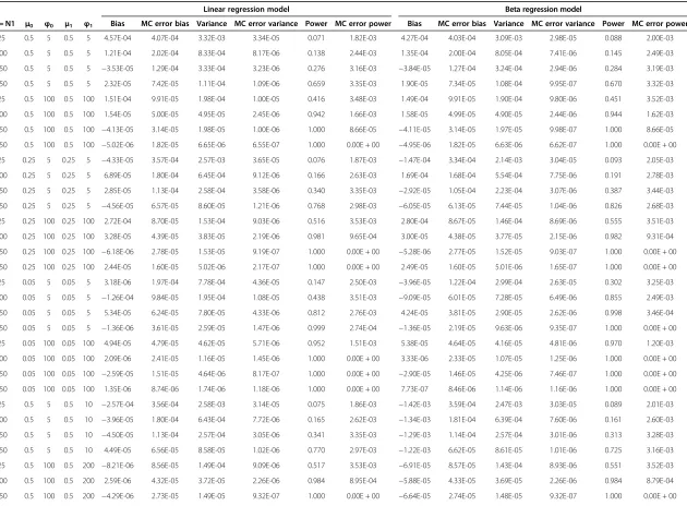
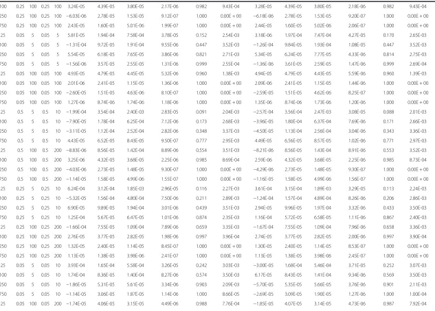
Table 4 Mean estimates from 20000 replicate simulations of bias (MC error of bias), variance (MC error of variance) and power (MC error power), from the fitted linear, beta, variable-dispersion beta and fractional logit regression models estimated on the beta distributed response data (Power experiments)

N0 = N1 μ0 φ0 μ1 φ1 Bias MC error bias Variance MC error variance Power MC error power Bias MC error bias Variance MC error variance Power MC error power

25 0.5 5 0.5 5 4.57E-04 4.07E-04 3.32E-03 3.34E-05 0.071 1.82E-03 4.27E-04 4.03E-04 3.09E-03 2.98E-05 0.088 2.00E-03

100 0.5 5 0.5 5 1.21E-04 2.02E-04 8.33E-04 8.17E-06 0.138 2.44E-03 1.35E-04 2.00E-04 8.05E-04 7.41E-06 0.145 2.49E-03

250 0.5 5 0.5 5 ₋3.53E-05 1.29E-04 3.33E-04 3.23E-06 0.276 3.16E-03 ₋3.84E-05 1.27E-04 3.24E-04 2.94E-06 0.284 3.19E-03

750 0.5 5 0.5 5 2.32E-05 7.42E-05 1.11E-04 1.09E-06 0.659 3.35E-03 1.90E-05 7.34E-05 1.08E-04 9.95E-07 0.670 3.32E-03

25 0.5 100 0.5 100 1.51E-04 9.91E-05 1.98E-04 1.00E-05 0.416 3.48E-03 1.49E-04 9.91E-05 1.90E-04 9.80E-06 0.451 3.52E-03

100 0.5 100 0.5 100 1.54E-05 5.00E-05 4.95E-05 2.45E-06 0.942 1.66E-03 1.58E-05 4.99E-05 4.90E-05 2.44E-06 0.944 1.62E-03

250 0.5 100 0.5 100 ₋4.13E-05 3.14E-05 1.98E-05 1.00E-06 1.000 8.66E-05 ₋4.11E-05 3.14E-05 1.97E-05 9.98E-07 1.000 8.66E-05

750 0.5 100 0.5 100 ₋5.02E-06 1.82E-05 6.65E-06 6.55E-07 1.000 0.00E + 00 ₋4.95E-06 1.82E-05 6.63E-06 6.62E-07 1.000 0.00E + 00

25 0.25 5 0.25 5 ₋4.33E-05 3.57E-04 2.57E-03 3.65E-05 0.076 1.87E-03 ₋1.47E-04 3.34E-04 2.14E-03 3.04E-05 0.093 2.05E-03

100 0.25 5 0.25 5 6.89E-05 1.80E-04 6.45E-04 9.12E-06 0.166 2.63E-03 1.69E-04 1.68E-04 5.54E-04 7.75E-06 0.191 2.78E-03

250 0.25 5 0.25 5 2.85E-05 1.13E-04 2.58E-04 3.58E-06 0.340 3.35E-03 ₋2.92E-05 1.05E-04 2.23E-04 3.07E-06 0.387 3.44E-03

750 0.25 5 0.25 5 ₋4.56E-05 6.57E-05 8.60E-05 1.21E-06 0.768 2.98E-03 ₋6.05E-05 6.13E-05 7.44E-05 1.04E-06 0.826 2.68E-03

25 0.25 100 0.25 100 2.72E-04 8.70E-05 1.53E-04 9.03E-06 0.516 3.53E-03 2.80E-04 8.67E-05 1.46E-04 8.69E-06 0.555 3.51E-03

100 0.25 100 0.25 100 3.28E-05 4.39E-05 3.83E-05 2.19E-06 0.981 9.65E-04 3.00E-05 4.38E-05 3.77E-05 2.15E-06 0.982 9.31E-04

250 0.25 100 0.25 100 ₋6.18E-06 2.78E-05 1.53E-05 9.19E-07 1.000 0.00E + 00 ₋5.28E-06 2.77E-05 1.52E-05 9.03E-07 1.000 0.00E + 00

750 0.25 100 0.25 100 2.44E-05 1.60E-05 5.02E-06 2.17E-07 1.000 0.00E + 00 2.49E-05 1.60E-05 5.01E-06 1.65E-07 1.000 0.00E + 00

25 0.05 5 0.05 5 3.18E-06 1.97E-04 7.78E-04 4.36E-05 0.147 2.50E-03 ₋3.96E-05 1.22E-04 2.99E-04 2.63E-05 0.302 3.25E-03

100 0.05 5 0.05 5 ₋1.26E-04 9.84E-05 1.95E-04 1.08E-05 0.438 3.51E-03 ₋9.09E-05 6.01E-05 7.28E-05 6.49E-06 0.855 2.49E-03

250 0.05 5 0.05 5 5.34E-05 6.24E-05 7.80E-05 4.33E-06 0.812 2.76E-03 4.24E-05 3.81E-05 2.90E-05 2.62E-06 0.998 3.46E-04

750 0.05 5 0.05 5 ₋1.36E-06 3.61E-05 2.59E-05 1.47E-06 0.999 2.74E-04 ₋1.36E-05 2.19E-05 9.63E-06 9.35E-07 1.000 0.00E + 00

25 0.05 100 0.05 100 4.94E-05 4.79E-05 4.62E-05 5.71E-06 0.952 1.51E-03 5.38E-05 4.64E-05 4.16E-05 4.81E-06 0.970 1.20E-03

100 0.05 100 0.05 100 2.09E-06 2.41E-05 1.16E-05 1.45E-06 1.000 0.00E + 00 3.33E-06 2.33E-05 1.07E-05 1.25E-06 1.000 0.00E + 00

250 0.05 100 0.05 100 ₋2.59E-05 1.51E-05 4.64E-06 8.17E-07 1.000 0.00E + 00 ₋2.90E-05 1.46E-05 4.25E-06 7.46E-07 1.000 0.00E + 00

750 0.05 100 0.05 100 1.35E-06 8.74E-06 1.74E-06 1.18E-06 1.000 0.00E + 00 7.73E-07 8.46E-06 1.14E-06 1.16E-06 1.000 0.00E + 00

25 0.5 5 0.5 10 ₋2.57E-04 3.56E-04 2.58E-03 3.14E-05 0.075 1.86E-03 ₋1.42E-03 3.59E-04 2.47E-03 3.03E-05 0.089 2.01E-03

100 0.5 5 0.5 10 ₋3.96E-05 1.80E-04 6.43E-04 7.72E-06 0.165 2.62E-03 ₋1.34E-03 1.81E-04 6.39E-04 7.60E-06 0.161 2.60E-03

250 0.5 5 0.5 10 ₋4.50E-05 1.13E-04 2.57E-04 3.05E-06 0.341 3.35E-03 ₋1.29E-03 1.14E-04 2.57E-04 3.01E-06 0.313 3.28E-03

750 0.5 5 0.5 10 4.49E-05 6.56E-05 8.58E-05 1.02E-06 0.770 2.97E-03 ₋1.22E-03 6.62E-05 8.61E-05 1.01E-06 0.725 3.16E-03

25 0.5 100 0.5 200 ₋8.21E-06 8.56E-05 1.49E-04 9.09E-06 0.517 3.53E-03 ₋6.91E-05 8.57E-05 1.43E-04 8.93E-06 0.551 3.52E-03

100 0.5 100 0.5 200 2.59E-06 4.32E-05 3.72E-05 2.26E-06 0.984 8.95E-04 ₋5.88E-05 4.33E-05 3.69E-05 2.26E-06 0.984 8.79E-04

250 0.5 100 0.5 200 ₋4.29E-06 2.73E-05 1.49E-05 9.32E-07 1.000 0.00E + 00 ₋6.64E-05 2.74E-05 1.48E-05 9.32E-07 1.000 0.00E + 00

Meaney

and

Moineddin

BMC

Medical

Research

Methodolog

y

2014,

14

:14

Page

13

of

22

http://ww

w.biomedce

ntral.com/1

(14)

Table 4 Mean estimates from 20000 replicate simulations of bias (MC error of bias), variance (MC error of variance) and power (MC error power), from the fitted linear, beta, variable-dispersion beta and fractional logit regression models estimated on the beta distributed response data (Power experiments) (Continued)

750 0.5 100 0.5 200 −1.16E-05 1.58E-05 5.00E-06 1.54E-07 1.000 0.00E + 00 −7.40E-05 1.58E-05 5.00E-06 1.56E-07 1.000 0.00E + 00

25 0.25 5 0.25 10 3.61E-04 3.15E-04 1.97E-03 3.36E-05 0.098 2.10E-03 2.22E-02 2.99E-04 1.73E-03 2.89E-05 0.223 2.94E-03

100 0.25 5 0.25 10 −1.24E-04 1.57E-04 4.94E-04 8.31E-06 0.201 2.83E-03 2.26E-02 1.49E-04 4.48E-04 7.27E-06 0.613 3.44E-03

250 0.25 5 0.25 10 2.94E-05 9.96E-05 1.97E-04 3.33E-06 0.430 3.50E-03 2.29E-02 9.42E-05 1.80E-04 2.90E-06 0.945 1.62E-03

750 0.25 5 0.25 10 1.16E-04 5.72E-05 6.59E-05 1.12E-06 0.867 2.40E-03 2.31E-02 5.45E-05 6.02E-05 9.81E-07 1.000 0.00E + 00

25 0.25 100 0.25 200 −1.67E-04 7.55E-05 1.14E-04 8.12E-06 0.625 3.42E-03 9.73E-04 7.53E-05 1.10E-04 7.94E-06 0.695 3.26E-03

100 0.25 100 0.25 200 2.74E-05 3.77E-05 2.85E-05 2.00E-06 0.997 4.12E-04 1.20E-03 3.76E-05 2.84E-05 1.99E-06 0.999 2.69E-04

250 0.25 100 0.25 200 1.30E-05 2.40E-05 1.14E-05 8.55E-07 1.000 0.00E + 00 1.20E-03 2.39E-05 1.14E-05 8.51E-07 1.000 0.00E + 00

750 0.25 100 0.25 200 1.13E-05 1.38E-05 3.98E-06 2.35E-07 1.000 0.00E + 00 1.20E-03 1.38E-05 3.99E-06 1.98E-07 1.000 0.00E + 00

25 0.05 5 0.05 10 −3.00E-05 1.68E-04 5.69E-04 3.79E-05 0.229 2.97E-03 2.24E-02 1.10E-04 2.79E-04 2.19E-05 0.867 2.40E-03

100 0.05 5 0.05 10 6.17E-05 8.43E-05 1.42E-04 9.39E-06 0.561 3.51E-03 2.32E-02 5.35E-05 6.95E-05 5.41E-06 1.000 0.00E + 00

250 0.05 5 0.05 10 −5.70E-05 5.35E-05 5.69E-05 3.77E-06 0.899 2.13E-03 2.33E-02 3.41E-05 2.78E-05 2.18E-06 1.000 0.00E + 00

750 0.05 5 0.05 10 −2.69E-05 3.09E-05 1.90E-05 1.27E-06 1.000 1.00E-04 2.34E-02 1.96E-05 9.28E-06 7.90E-07 1.000 0.00E + 00

25 0.05 100 0.05 200 −1.85E-05 4.07E-05 3.27E-05 4.82E-06 0.984 8.91E-04 2.03E-03 3.96E-05 3.18E-05 4.38E-06 0.997 4.06E-04

100 0.05 100 0.05 200 1.15E-05 2.02E-05 8.15E-06 1.23E-06 1.000 0.00E + 00 2.14E-03 1.96E-05 8.17E-06 1.14E-06 1.000 0.00E + 00

250 0.05 100 0.05 200 −1.34E-05 1.28E-05 3.16E-06 7.35E-07 1.000 0.00E + 00 2.13E-03 1.25E-05 3.17E-06 7.53E-07 1.000 0.00E + 00

750 0.05 100 0.05 200 9.87E-06 7.31E-06 1.00E-06 0.00E + 00 1.000 0.00E + 00 2.16E-03 7.09E-06 1.00E-06 0.00E + 00 1.000 0.00E + 00

N0 = N1 μ0 φ0 μ1 φ1 Bias MC error bias Variance MC error variance Power MC error power Bias MC error bias Variance MC error variance Power MC error power

25 0.5 5 0.5 5 4.80E-04 4.04E-04 3.08E-03 2.96E-05 0.090 2.02E-03 4.57E-04 4.07E-04 3.19E-03 3.27E-05 0.085 1.97E-03

100 0.5 5 0.5 5 1.41E-04 2.00E-04 8.04E-04 7.40E-06 0.146 2.50E-03 1.21E-04 2.02E-04 8.24E-04 8.13E-06 0.142 2.47E-03

250 0.5 5 0.5 5 −3.46E-05 1.27E-04 3.24E-04 2.94E-06 0.284 3.19E-03 −3.53E-05 1.29E-04 3.32E-04 3.23E-06 0.279 3.17E-03

750 0.5 5 0.5 5 2.07E-05 7.34E-05 1.08E-04 9.95E-07 0.671 3.32E-03 2.32E-05 7.42E-05 1.11E-04 1.09E-06 0.660 3.35E-03

25 0.5 100 0.5 100 1.49E-04 9.91E-05 1.90E-04 9.80E-06 0.451 3.52E-03 1.51E-04 9.91E-05 1.90E-04 9.82E-06 0.451 3.52E-03

100 0.5 100 0.5 100 1.57E-05 5.00E-05 4.90E-05 2.44E-06 0.944 1.62E-03 1.54E-05 5.00E-05 4.90E-05 2.44E-06 0.944 1.62E-03

250 0.5 100 0.5 100 −4.11E-05 3.14E-05 1.97E-05 9.98E-07 1.000 8.66E-05 −4.13E-05 3.14E-05 1.97E-05 9.97E-07 1.000 8.66E-05

750 0.5 100 0.5 100 −5.02E-06 1.82E-05 6.63E-06 6.62E-07 1.000 0.00E + 00 −5.02E-06 1.82E-05 6.63E-06 6.61E-07 1.000 0.00E + 00

25 0.25 5 0.25 5 −1.33E-05 3.54E-04 2.40E-03 3.18E-05 0.091 2.03E-03 −4.33E-05 3.57E-04 2.47E-03 3.58E-05 0.090 2.02E-03

100 0.25 5 0.25 5 1.27E-04 1.78E-04 6.24E-04 8.14E-06 0.173 2.68E-03 6.89E-05 1.80E-04 6.39E-04 9.08E-06 0.171 2.66E-03

250 0.25 5 0.25 5 2.63E-06 1.12E-04 2.51E-04 3.21E-06 0.349 3.37E-03 2.85E-05 1.13E-04 2.57E-04 3.57E-06 0.343 3.36E-03

750 0.25 5 0.25 5 −5.12E-05 6.50E-05 8.41E-05 1.09E-06 0.777 2.94E-03 −4.56E-05 6.57E-05 8.59E-05 1.21E-06 0.769 2.98E-03

25 0.25 100 0.25 100 2.73E-04 8.70E-05 1.47E-04 8.76E-06 0.552 3.52E-03 2.72E-04 8.70E-05 1.47E-04 8.85E-06 0.551 3.52E-03

Meaney

and

Moineddin

BMC

Medical

Research

Methodolog

y

2014,

14

:14

Page

14

of

22

http://ww

w.biomedce

ntral.com/1

(15)

100 0.25 100 0.25 100 3.24E-05 4.39E-05 3.80E-05 2.17E-06 0.982 9.43E-04 3.28E-05 4.39E-05 3.80E-05 2.18E-06 0.982 9.43E-04

250 0.25 100 0.25 100 −6.03E-06 2.78E-05 1.53E-05 9.12E-07 1.000 0.00E + 00 −6.18E-06 2.78E-05 1.53E-05 9.20E-07 1.000 0.00E + 00

750 0.25 100 0.25 100 2.43E-05 1.60E-05 5.01E-06 1.99E-07 1.000 0.00E + 00 2.44E-05 1.60E-05 5.02E-06 2.06E-07 1.000 0.00E + 00

25 0.05 5 0.05 5 5.81E-05 1.94E-04 7.58E-04 3.78E-05 0.152 2.54E-03 3.18E-06 1.97E-04 7.47E-04 4.27E-05 0.170 2.65E-03

100 0.05 5 0.05 5 −1.31E-04 9.72E-05 1.91E-04 9.55E-06 0.447 3.52E-03 −1.26E-04 9.84E-05 1.93E-04 1.08E-05 0.447 3.52E-03

250 0.05 5 0.05 5 5.54E-05 6.18E-05 7.65E-05 3.86E-06 0.821 2.71E-03 5.34E-05 6.24E-05 7.77E-05 4.33E-06 0.814 2.75E-03

750 0.05 5 0.05 5 −1.56E-06 3.57E-05 2.55E-05 1.31E-06 0.999 2.55E-04 −1.36E-06 3.61E-05 2.59E-05 1.47E-06 0.999 2.69E-04

25 0.05 100 0.05 100 4.93E-05 4.79E-05 4.45E-05 5.32E-06 0.960 1.38E-03 4.94E-05 4.79E-05 4.43E-05 5.59E-06 0.960 1.39E-03

100 0.05 100 0.05 100 2.01E-06 2.41E-05 1.15E-05 1.36E-06 1.000 0.00E + 00 2.09E-06 2.41E-05 1.15E-05 1.44E-06 1.000 0.00E + 00

250 0.05 100 0.05 100 −2.60E-05 1.51E-05 4.63E-06 8.10E-07 1.000 0.00E + 00 −2.59E-05 1.51E-05 4.62E-06 8.25E-07 1.000 0.00E + 00

750 0.05 100 0.05 100 1.27E-06 8.74E-06 1.74E-06 1.18E-06 1.000 0.00E + 00 1.35E-06 8.74E-06 1.73E-06 1.20E-06 1.000 0.00E + 00

25 0.5 5 0.5 10 −1.99E-04 3.54E-04 2.40E-03 2.83E-05 0.091 2.04E-03 −2.57E-04 3.56E-04 2.47E-03 3.08E-05 0.088 2.01E-03

100 0.5 5 0.5 10 −7.90E-05 1.78E-04 6.25E-04 7.12E-06 0.173 2.68E-03 −3.96E-05 1.80E-04 6.37E-04 7.69E-06 0.171 2.66E-03

250 0.5 5 0.5 10 −3.11E-05 1.12E-04 2.52E-04 2.82E-06 0.348 3.37E-03 −4.50E-05 1.13E-04 2.56E-04 3.04E-06 0.343 3.36E-03

750 0.5 5 0.5 10 4.43E-05 6.52E-05 8.43E-05 9.50E-07 0.777 2.95E-03 4.49E-05 6.56E-05 8.57E-05 1.02E-06 0.771 2.97E-03

25 0.5 100 0.5 200 −8.83E-06 8.56E-05 1.42E-04 8.89E-06 0.554 3.51E-03 −8.21E-06 8.56E-05 1.43E-04 8.91E-06 0.553 3.52E-03

100 0.5 100 0.5 200 3.25E-06 4.32E-05 3.68E-05 2.25E-06 0.985 8.69E-04 2.59E-06 4.32E-05 3.68E-05 2.25E-06 0.985 8.73E-04

250 0.5 100 0.5 200 −4.03E-06 2.73E-05 1.48E-05 9.30E-07 1.000 0.00E + 00 −4.29E-06 2.73E-05 1.48E-05 9.30E-07 1.000 0.00E + 00

750 0.5 100 0.5 200 −1.14E-05 1.58E-05 4.99E-06 1.55E-07 1.000 0.00E + 00 −1.16E-05 1.58E-05 4.99E-06 1.56E-07 1.000 0.00E + 00

25 0.25 5 0.25 10 6.24E-04 3.12E-04 1.85E-03 2.96E-05 0.116 2.27E-03 3.61E-04 3.15E-04 1.89E-03 3.29E-05 0.113 2.24E-03

100 0.25 5 0.25 10 −5.32E-05 1.56E-04 4.80E-04 7.50E-06 0.211 2.89E-03 −1.24E-04 1.57E-04 4.89E-04 8.26E-06 0.206 2.86E-03

250 0.25 5 0.25 10 6.90E-05 9.89E-05 1.94E-04 3.01E-06 0.439 3.51E-03 2.94E-05 9.96E-05 1.97E-04 3.32E-06 0.433 3.50E-03

750 0.25 5 0.25 10 1.25E-04 5.67E-05 6.47E-05 1.01E-06 0.874 2.35E-03 1.16E-04 5.72E-05 6.58E-05 1.11E-06 0.867 2.40E-03

25 0.25 100 0.25 200 −1.66E-04 7.55E-05 1.09E-04 7.89E-06 0.659 3.35E-03 −1.67E-04 7.55E-05 1.09E-04 7.96E-06 0.658 3.36E-03

100 0.25 100 0.25 200 2.76E-05 3.77E-05 2.82E-05 1.98E-06 0.997 3.96E-04 2.74E-05 3.77E-05 2.82E-05 2.00E-06 0.997 3.90E-04

250 0.25 100 0.25 200 1.32E-05 2.40E-05 1.14E-05 8.45E-07 1.000 0.00E + 00 1.30E-05 2.40E-05 1.14E-05 8.53E-07 1.000 0.00E + 00

750 0.25 100 0.25 200 1.13E-05 1.38E-05 3.98E-06 2.41E-07 1.000 0.00E + 00 1.13E-05 1.38E-05 3.98E-06 2.45E-07 1.000 0.00E + 00

25 0.05 5 0.05 10 3.93E-04 1.65E-04 5.58E-04 3.26E-05 0.242 3.03E-03 −3.00E-05 1.68E-04 5.46E-04 3.71E-05 0.252 3.07E-03

100 0.05 5 0.05 10 1.74E-04 8.36E-05 1.40E-04 8.27E-06 0.574 3.50E-03 6.17E-05 8.43E-05 1.41E-04 9.34E-06 0.569 3.50E-03

250 0.05 5 0.05 10 −1.86E-05 5.31E-05 5.61E-05 3.34E-06 0.903 2.09E-03 −5.70E-05 5.35E-05 5.66E-05 3.76E-06 0.901 2.11E-03

750 0.05 5 0.05 10 −1.14E-05 3.06E-05 1.87E-05 1.14E-06 1.000 8.66E-05 −2.69E-05 3.09E-05 1.90E-05 1.27E-06 1.000 1.00E-04

25 0.05 100 0.05 200 −1.74E-05 4.06E-05 3.15E-05 4.49E-06 0.988 7.76E-04 −1.85E-05 4.07E-05 3.14E-05 4.73E-06 0.987 7.92E-04

Meaney

and

Moineddin

BMC

Medical

Research

Methodolog

y

2014,

14

:14

Page

15

of

22

http://ww

w.biomedce

ntral.com/1

(16)

100 0.05 100 0.05 200 1.21E-05 2.02E-05 8.08E-06 1.16E-06 1.000 0.00E + 00 1.15E-05 2.02E-05 8.07E-06 1.23E-06 1.000 0.00E + 00

250 0.05 100 0.05 200 −1.32E-05 1.28E-05 3.14E-06 6.89E-07 1.000 0.00E + 00 −1.34E-05 1.28E-05 3.15E-06 7.11E-07 1.000 0.00E + 00

750 0.05 100 0.05 200 9.78E-06 7.31E-06 1.00E-06 0.00E + 00 1.000 0.00E + 00 9.87E-06 7.31E-06 1.00E-06 0.00E + 00 1.000 0.00E + 00

The first 24 rows of the Table describe experiments where the dispersion parameter does not vary as a function of group membership; whereas, in the bottom 24 rows of the Table the dispersion parameter varies as a function of group membership. Rows 1–8 (and 25–32) correspond to simulated experiments where the mass of the distribution is near 0.50, rows 9–16 (and 33–40) correspond to simulated experiments where the mass of the distribution is centered near 0.25, and finally rows 17–24 (and 41–48) correspond to simulated experiments where the mass of the distribution is near 0.05.

Δ= 0.025 (power experiments).

Power refers to the proportion of null hypothesis rejected.

Meaney

and

Moineddin

BMC

Medical

Research

Methodolog

y

2014,

14

:14

Page

16

of

22

http://ww

w.biomedce

ntral.com/1

(17)

Table 5 Mean estimates from 20000 replicate simulations of bias (MC error of bias), variance (MC error of variance) and type-1 error (MC error type-1 error), from the fitted linear, beta, variable-dispersion beta and fractional logit regression models estimated on the multinomial distributed response data (Type-1 error experiments)

N0 = N1 E(Y0) E(Y1) Bias MC error bias Variance MC error variance Type-1 Error MC Error Type-1 Error Bias MC error bias Variance MC error variance Type-1 Error MC Error Type-1 Error

25 0.5 0.5 −6.22E-04 2.64E-04 1.40E-03 3.04E-05 0.048 0.002 −6.48E-04 2.72E-04 1.39E-03 3.04E-05 0.062 0.002

100 0.5 0.5 8.00E-06 1.32E-04 3.50E-04 7.51E-06 0.049 0.002 −2.97E-06 1.37E-04 3.61E-04 7.68E-06 0.055 0.002

250 0.5 0.5 1.07E-04 8.33E-05 1.40E-04 3.02E-06 0.051 0.002 1.09E-04 8.60E-05 1.46E-04 3.10E-06 0.053 0.002

750 0.5 0.5 −3.01E-06 4.84E-05 4.67E-05 1.01E-06 0.051 0.002 −2.56E-06 4.99E-05 4.87E-05 1.03E-06 0.054 0.002

25 0.215 0.215 −4.46E-04 3.72E-04 2.74E-03 3.41E-05 0.051 0.002 −3.06E-04 2.80E-04 1.82E-03 3.12E-05 0.037 0.001

100 0.215 0.215 5.06E-05 1.85E-04 6.86E-04 8.38E-06 0.050 0.002 −2.96E-05 1.38E-04 4.64E-04 7.95E-06 0.030 0.001

250 0.215 0.215 1.18E-04 1.17E-04 2.74E-04 3.31E-06 0.051 0.002 1.19E-04 8.69E-05 1.86E-04 3.17E-06 0.030 0.001

750 0.215 0.215 −1.10E-05 6.78E-05 9.13E-05 1.11E-06 0.050 0.002 −1.93E-05 5.02E-05 6.20E-05 1.06E-06 0.029 0.001

N0 = N1 E(Y0) E(Y1) Bias MC error bias Variance MC error variance Type-1 Error MC Error Type-1 Error Bias MC error bias Variance MC error variance Type-1 Error MC Error Type-1 Error

25 0.5 0.5 −6.43E-04 2.71E-04 1.38E-03 3.02E-05 0.063 0.002 −6.22E-04 2.64E-04 1.34E-03 2.98E-05 0.060 0.002

100 0.5 0.5 −4.54E-07 1.37E-04 3.61E-04 7.66E-06 0.055 0.002 8.00E-06 1.32E-04 3.46E-04 7.47E-06 0.052 0.002

250 0.5 0.5 1.09E-04 8.59E-05 1.45E-04 3.10E-06 0.053 0.002 1.07E-04 8.33E-05 1.39E-04 3.01E-06 0.052 0.002

750 0.5 0.5 −2.57E-06 4.99E-05 4.87E-05 1.03E-06 0.054 0.002 −3.01E-06 4.84E-05 4.66E-05 1.01E-06 0.052 0.002

25 0.215 0.215 −3.94E-04 3.51E-04 2.19E-03 3.13E-05 0.072 0.002 −4.46E-04 3.72E-04 2.63E-03 3.34E-05 0.062 0.002

100 0.215 0.215 5.99E-05 1.74E-04 5.63E-04 7.95E-06 0.061 0.002 5.06E-05 1.85E-04 6.79E-04 8.33E-06 0.053 0.002

250 0.215 0.215 1.08E-04 1.10E-04 2.26E-04 3.16E-06 0.060 0.002 1.18E-04 1.17E-04 2.73E-04 3.30E-06 0.053 0.002

750 0.215 0.215 −1.64E-06 6.37E-05 7.55E-05 1.06E-06 0.059 0.002 −1.10E-05 6.78E-05 9.12E-05 1.11E-06 0.050 0.002

Response variables were generated from a discrete multinomial distribution with probability mass observed only on points in (0,1). Multinomial response probabilities for this experiment are given in Table2above.

Δ= 0 (type-1 error experiments).

Type-1 error refers to the proportion of null hypothesis rejected (expected 0.05).

Meaney

and

Moineddin

BMC

Medical

Research

Methodolog

y

2014,

14

:14

Page

17

of

22

http://ww

w.biomedce

ntral.com/1

(18)

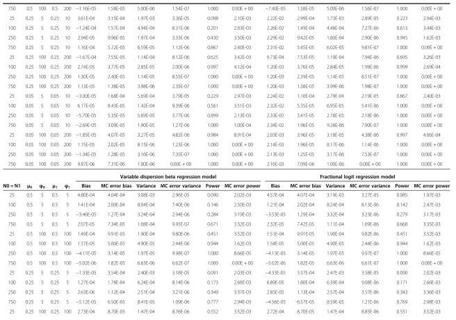
Table 6 Mean estimates from 20000 replicate simulations of bias (MC error of bias), variance (MC Error Variance), and Power (MC Error Power), from the fitted linear, beta, variable-dispersion beta and fractional logit regression models estimated on the multinomial distributed response data (Power experiments)

N0 = N1 E(Y0) E(Y1) Bias MC error bias Variance MC error variance Power MC error power Bias MC error bias Variance MC error variance Power MC error power

25 0.5 0.6 −1.36E-04 2.63E-04 1.40E-03 3.04E-05 0.745 0.003 2.32E-03 2.76E-04 1.44E-03 3.22E-05 0.769 0.003

100 0.5 0.6 −2.17E-04 1.33E-04 3.50E-04 7.54E-06 1.000 0.000 2.37E-03 1.39E-04 3.72E-04 8.18E-06 1.000 0.000

250 0.5 0.6 −5.06E-05 8.32E-05 1.40E-04 3.02E-06 1.000 0.000 2.55E-03 8.73E-05 1.50E-04 3.29E-06 1.000 0.000

750 0.5 0.6 −8.70E-05 4.85E-05 4.66E-05 1.01E-06 1.000 0.000 2.55E-03 5.08E-05 5.02E-05 1.10E-06 1.000 0.000

25 0.215 0.315 2.82E-04 3.70E-04 2.75E-03 3.42E-05 0.466 0.004 1.35E-02 2.96E-04 2.02E-03 3.04E-05 0.725 0.003

100 0.215 0.315 6.30E-06 1.84E-04 6.85E-04 8.36E-06 0.966 0.001 1.36E-02 1.46E-04 5.17E-04 7.65E-06 1.000 0.000

250 0.215 0.315 1.87E-05 1.17E-04 2.74E-04 3.31E-06 1.000 0.000 1.37E-02 9.28E-05 2.08E-04 3.04E-06 1.000 0.000

750 0.215 0.315 1.02E-04 6.74E-05 9.14E-05 1.10E-06 1.000 0.000 1.38E-02 5.33E-05 6.94E-05 1.02E-06 1.000 0.000

N0 = N1 E(Y0) E(Y1) Bias MC error bias Variance MC error variance Power MC error power Bias MC error bias Variance MC error variance Power MC error power

25 0.5 0.6 1.77E-03 2.73E-04 1.43E-03 3.20E-05 0.767 0.003 −1.36E-04 2.63E-04 1.35E-03 2.98E-05 0.774 0.003

100 0.5 0.6 1.86E-03 1.38E-04 3.72E-04 8.16E-06 1.000 0.000 −2.17E-04 1.33E-04 3.46E-04 7.50E-06 1.000 0.000

250 0.5 0.6 2.05E-03 8.64E-05 1.50E-04 3.28E-06 1.000 0.000 −5.06E-05 8.32E-05 1.39E-04 3.01E-06 1.000 0.000

750 0.5 0.6 2.05E-03 5.04E-05 5.02E-05 1.10E-06 1.000 0.000 −8.70E-05 4.85E-05 4.66E-05 1.01E-06 1.000 0.000

25 0.215 0.315 3.33E-03 3.55E-04 2.21E-03 3.07E-05 0.589 0.003 2.82E-04 3.70E-04 2.64E-03 3.35E-05 0.501 0.004

100 0.215 0.315 3.10E-03 1.77E-04 5.68E-04 7.71E-06 0.987 0.001 6.30E-06 1.84E-04 6.78E-04 8.32E-06 0.967 0.001

250 0.215 0.315 3.14E-03 1.12E-04 2.28E-04 3.07E-06 1.000 0.000 1.87E-05 1.17E-04 2.73E-04 3.30E-06 1.000 0.000

750 0.215 0.315 3.22E-03 6.45E-05 7.64E-05 1.03E-06 1.000 0.000 1.02E-04 6.74E-05 9.13E-05 1.11E-06 1.000 0.000

Response variables were generated from a discrete multinomial distribution with probability mass observed only on points in (0,1). Multinomial response probabilities for this experiment are given in Table2above.

Δ= 0.10 (power experiments).

Power refers to the proportion of null hypothesis rejected.

Meaney

and

Moineddin

BMC

Medical

Research

Methodolog

y

2014,

14

:14

Page

18

of

22

http://ww

w.biomedce

ntral.com/1