Vol. 9, No. 1, 2017 Article ID IJIM-00713, 20 pages Research Article
A Hybrid Heuristic Algorithm to Solve Capacitated Location-routing
Problem With Fuzzy Demands
A. Nadizadeh ∗†, A. Sadegheih‡, A. Sabzevari Zadeh §
Received Date: 2015-06-09 Revised Date: 2015-09-13 Accepted Date: 2016-05-21 ————————————————————————————————–
Abstract
In this paper, the capacitated location-routing problem with fuzzy demands (CLRP-FD) is considered. The CLRP-FD is composed of two well-known problems: facility location problem and vehicle routing problem. The problem has many real-life applications of which some have been addressed in the literature such as management of hazardous wastes and food and drink distribution. In CLRP-FD, a set of customers with fuzzy demands should be supplied by a fleet of vehicles that start and end their tours at a single depot. Moreover, the vehicles and the depots have a limited capacity. To model this problem, a fuzzy chance-constrained programming is designed based on fuzzy credibility theory. To solve the CLRP-FD, a hybrid heuristic algorithm (HHA) including two main phases is proposed. In the first phase, an initial population of solutions is generated by the greedy clustering method (GCM) obtained from the literature of the problem, while in the second phase, a genetic algorithm is applied for further improvement of the solutions of first phase. While the first phase of the HHA consists of four steps, the second phase includes two main steps. To achieve the best value of the major parameter of the model, named dispatcher preference index, and to analyze its influence on the changes of the final solution, numerical experiments with different sizes on the number of customers and candidate depots are carried out. The computational results show that the HHA is efficient so that it has improved all solutions that obtained from the GCM. Finally, performance of the proposed model to the similar model exists in the literature is evaluated by several standard test problems of the CLRP.
Keywords: Capacitated location-routing problem; Fuzzy demand; Credibility theory; Stochastic sim-ulation; Fuzzy-chance constrained programming; Genetic algorithm.
—————————————————————————————————–
1
Introduction
E
vtheir desired products with less waiting timeer increasing demand of customers to receive ∗Corresponding author. [email protected], Tel: +98(913)2551763†Department of Industrial Engineering, Faculty of En-gineering, Ardakan University, Ardakan, Iran.
‡Industrial Engineering Department, Faculty of Engi-neering, Yazd University, Yazd, Iran.
§Industrial Engineering Department, Faculty of Engi-neering, Shahed University, Tehran, Iran.
and competitive prices, make the logistics as the main problem in supply chain management. In recent years, efficient, reliable, and flexible de-cisions on location of depots and vehicle rout-ings are of vital importance to managers [23,57]. Many researchers indicated that if the routes are ignored while locating the depots, the costs of dis-tribution systems might be immoderate [22,42]. At the first attempt, Salhi and Rand [44] showed that solving the location problem without route consideration may lead to a sub-optimal solution. The location-routing problem (LRP) overcomes
this drawback through making the location and routing decisions, simultaneously. The LRP is defined as a facility location problem (FLP) that solves the vehicle routing problem (VRP), simul-taneously [26, 47]. Since both problems belong to the class of NP-hard problem, the LRP is also an NP-hard problem [4, 6, 60]. The LRP is applicable for a wide variety of fields such as food and drink distribution, newspapers delivery, waste collection, bill delivery, military applica-tions, parcel delivery and various consumer goods distribution, etc. [29, 45]. In the capacitated location-routing problem (CLRP), the problem is limited with the vehicles and the depots’ ca-pacities to supply the customers. Furthermore, the customers must only be supplied by a single vehicle which means that the vehicle meets ev-ery customer in a tour only once. A homogenous fleet of vehicles transports the products with spe-cific capacity from depots to the customers and returns there as soon as finishing the entire tour. The objectives in the CLRP are to determine the location of depots and a set of customers to be assigned to each depot as well as the distribution routes [9, 32, 38]. Since the CLRP is an NP-hard problem, some authors have employed ap-proximation heuristic algorithms for solving that [30, 54]. In this kind of problems, the solution time increases exponentially as with an increase in the size of the problem, while an exact algo-rithm is applied to solve them. For this reason, most papers in the field of CLRP have only fo-cused on new solution methods that are often based on heuristic or meta-heuristic approaches [36]. Some reviews on solution methods of the CLRP exist in literature that can be found in [12,13,34,43].
Nagy and Salhi [34] classified the heuristics into four different types as follows: sequential, clustering-based, iterative, and hierarchical. Se-quential methods solve the location problem by minimizing the sum of facility to customer dis-tance and the routing problem based on the selected depots sequentially. Clustering-based methods partition the customers into clusters and then find a depot for each cluster [46, 4]. The VRP is then solved for each cluster. It-erative methods decompose the LRP into two sub-problems. Then, sub-problems are solved it-eratively by feeding information from one sub-problem to the other [53, 40, 13]. Hierarchical
methods consider the location problem as the main problem and the VRP as a subordinated problem [33,1].
Many heuristics that hybrid two different heuristic approaches are proposed in the litera-ture of the LRP. Since this study uses a two-phase approach to solve the problem, the similar works are summarized as follows:
Tuzun and Burke [50] proposed a two-phase tabu search (TS) approach for the LRP. One phase seeks a good facility configuration while the other one obtains a good routing for this config-uration. Wu et al. [53] presented a combined TS and simulated annealing (SA) decomposition approach to solve the multi-depot location rout-ing problem with multiple fleet types and lim-ited number of vehicles for each vehicle type. Lin et al. [27] developed a meta-heuristic approach based on threshold accepting (TA) and SA to as-sist in making decisions of facility location, vehi-cle routing and loading decision for bill delivery services in Hong Kong. Albareda-Sambola et al. [1] proposed another two-phase TS heuristic for the LRP which incurs not capacity constraints on vehicles. Wang et al. [52] proposed a two-phase hybrid heuristic which decomposes the LRP into location–allocation problem and vehicle routing problem. In the location phase, the TS was ap-plied to obtain the configuration of facility loca-tions. For each selected facility location, a vehicle routing problem was solved by ant colony opti-mization (ACO) in the routing phase. Bouhafs et al. [7] proposed a hybrid algorithm which com-bined the SA and ant colony system (ACS) to solve the CLRP. A good configuration of facilities was first found by the SA, and then the ACS was applied to construct the routings based on the configuration. These two ACO-related heuristics construct the routing problem and feedback the information for the facility selection phase.
[40] proposed a cooperative approach, which com-bines the Lagrangean relaxation and granular tabu search (GTS), to solve the CLRP. The algo-rithm alternates between a location sub-problem, solved by Lagrangean relaxation, and a multi-depot VRP, solved by the GTS. Duhamel et al. [13] presented a GRASP with evolutionary lo-cation search (GRASP-ELS) approach for the CLRP. Barreto et al. [4] integrated several hi-erarchical and non-hihi-erarchical clustering tech-niques in a sequential heuristic algorithm. Mari-nakis and Marinaki [30] developed a hybrid al-gorithm, which combined the particle swarm op-timization (PSO), multiple phase neighborhood search-greedy randomized adaptive search proce-dure (MPNS-GRASP), the expanding neighbor-hood search (ENS) and path relinking, to solve the LRP. Yu et al. [54] proposed a simulated an-nealing algorithm to solve the LRP. The LRP is generally considered as a deterministic case in the literature. A few researches have addressed fuzzy versions of the LRP [12]. Recently, fuzzy logic has been used to model many different problems. The need to use fuzzy logic in problems arises when-ever there are some vague or uncertain param-eters. Credibility theory has already been used in many problems with fuzzy parameters, in par-allel with some meta-heuristics. In the CLRP, some papers have been done with fuzzy vari-ables and credibility theory so far. The work of Zarandi et al. [58] was the first attempt to model the CLRP with fuzzy variables, using credibil-ity theory. They investigated a CLRP in which the travel time between every pair of nodes was a fuzzy variable. A simulation-embedded simu-lated annealing (SA) procedure was proposed in order to solve the problem. They tested the pro-posed method using standard test problems of the CLRP, and the results showed that their method was robust and could be used in real-world appli-cations. In the second work, Fazel Zarandi et al. [57] considered the LRP with time windows un-der uncertainty. It was assumed that demands of customers and travel times are fuzzy variables. In their work, a fuzzy chance-constrained pro-gramming model was designed using credibility theory and a simulation-embedded SA algorithm was presented in order to solve the problem. To initialize solutions of SA, a heuristic method based on fuzzy c-means clustering with Maha-lanobis distance and a sweep method were
costly, fuzzy logic is worthwhile in these prob-lems. As a result, the fuzzy set theory provides a convenient alternative framework for modeling real-world systems mathematically and offers sev-eral advantages to the use of heuristic approaches [3]. More precisely, some reasons for choosing fuzzy variables instead of probabilistic function in the customers’ demands are as follows:
1. The stochastic-probabilistic theory requires significant knowledge about the statistical distribution of the uncertain parameters. In contrast, fuzzy theory provides an efficient way to model imprecision even when no his-torical information is available.
2. The use of stochastic-probabilistic theory in-volves extensive computation and requires complete knowledge on the statistical distri-bution of the uncertain time-varying param-eters.
3. Fuzzy theory enables the use of fuzzy rules in heuristic algorithms.
4. Instead of optimizing the average behaviors, as in stochastic-probabilistic theory, fuzzy theory rather aims to find solutions where all constraints are satisfied to some extent with a sufficient level of confidence.
This paper contributes to the CLRP-FD in the following directions: (a) a fuzzy-chance con-strained programming (FCCP) is proposed based on credibility theory to model the problem which is slightly different from what previously investi-gated by researchers; (b) a hybrid heuristic algo-rithm (HHA) is integrated with stochastic sim-ulation to solve the problem; (c) the sensitivity analysis on the dispatcher preference index of the model is carried out; (d) the performance of the proposed model and the efficiency of the HHA are compared with both a commercial solver and a conventional approach by some numerical ex-amples. It is of interest to notice that, the HHA consists of two main phases and uses two well-known algorithms, ant colony system and genetic algorithm, which their efficiency have shown in solving the location-routing problems [10,48].
The remainder of this paper is organized as fol-lows: In Section 2, some basic concepts of the fuzzy theory are given. Section 3 introduces the CLRP-FD and presents a FCCP model using the
credibility theory. Details of the HHA to solve CLRP-FD are presented in Section 4. In Section
5, some numerical experiments are given to re-veal the performance of the model and proposed HHA. In the final section, the conclusion remarks of the paper are presented.
2
Fuzzy credibility theory
The concept of the fuzzy set was initiated by Zadeh [55] via the membership function. Then it has been well developed and applied in a wide variety of real problems. In order to measure a fuzzy event, the term fuzzy variable was intro-duced by Kaufmann [24], and then Zadeh [56] proposed the possibility measure theory of fuzzy variable. Although, possibility measure has been widely used, it has no self-duality property. How-ever, a self-dual measure is absolutely necessary in both theory and practice. In order to define a self-dual measure, a modified form of the possi-bility theory called credipossi-bility theory was founded by Liu [28] and has been recently applied by many scholars all around the world. Before proceed-ing with development of a fuzzy model for CLRP with credibility theory, a brief introduction to ba-sic concepts and definitions used in this paper is presented as follows:
Let Θ be a non-empty set, and P the power set of Θ. Each element in P is called an event, and ϕ is an empty set. In order to present an axiomatic definition of possibility, it is necessary to assign a number Pos{A} to each event A, which indicates the possibility that A will occur. To ensure that the number Pos{A} has certain mathematical properties, the following four axioms are approved [28]:
Axiom 2.1. Pos{Θ}= 1; Axiom 2.2. Pos{ϕ}= 0;
Axiom 2.3. For each Ai ∈p(Θ), Pos{ ∨
Ai} = supremumi Pos{Ai};
Axiom 2.4. If Θi is a non-empty set, and the
set function Posi{}; i = 1, 2, . . . , n, satisfies above three axioms, and Θ = Θ 1 × Θ 2× ...
× Θ n, then for each A ∈ p(Θ), Pos{A} =
supremum(θ1,θ2,...,θn)∈A Pos1 {θ1}
∧
Pos2{θ2}
∧ ... Posn{θn}.
credibility theory can be obtained from them [28].
Definition 2.1 Let (Θ, P(Θ), Pos) be a possi-bility space, and A be a set in p(Θ), then the ne-cessity measure of A is defined by Nec{A} = 1 – Pos{Ac}, that Ac is the complement of event A.
Definition 2.2 Let (Θ, P(Θ), Pos) be a possi-bility space, and A be a set in p(Θ), then the credibility measure of A is defined by Cr{A}= 12
(Pos{A} + Nes{A}).
Considering definition 2.2, the credibility of a fuzzy event is de?ned as the average of its pos-sibility and necessity. The credibility measure is self-dual. A fuzzy event may fail even though its possibility achieves 1, and holds even though its necessity is 0. However, the fuzzy event must hold if its credibility is 1, and fails if its credi-bility is 0. In fact, the law of credicredi-bility plays a role similar to what plays the role of probability in measurement theory for ordinary sets [15].
Now let consider a triangular fuzzy variable ˜d
= (d1, d2, d3) for demand of a customer, ˜d is described by its left boundary d1, and its right boundary d3. In other word, the dispatcher or manager can subjectively estimate, based on his experience or available data, the demand of a cus-tomer will not be less than d1 and greater than
d3. The value of d2 corresponding to a grade of membership of 1 can also be determined by a subjective estimate. If the actual demand of a customer is considered byr, the possibility, neces-sity and credibility are easily obtained as follows [14]:
Pos{d˜≥r}=
1, if r≤d2
d3−r
d3−d2, if d2≤r≤d3 0, if r≥d3
(2.1)
Nec{d˜≥r}=
1, if r≤d1
d2−r
d2−d1, if d1≤r≤d2 0, if r≥d2
(2.2)
Cr{d˜≥r}=
1, if r≤d1
2d2−d1−r
2(d2−d1), if d1≤r≤d2
d3−r
2(d3−d2), if d2≤r≤d3
0. if r≥d3
(2.3)
3
Problem
description
and
FCCP model for the
CLRP-FD
In the CLRP, demand of each customer should be supplied by a single vehicle and the total demand of customers in each route must not exceed the capacity of the vehicle. The vehicles start and end to the same depot, and total demand of the allocated customers must be less than or equal to the capacity of the depot. The objective of the problem is to minimize the total cost including opening costs of depots and routing costs.
In the CLRP-FD, in addition to the above as-sumptions, the demand of each customer is a tri-angular fuzzy number such as ˜d = (d1, d2, d3). To model the problem with credibility theory, the fuzzy number representing demand of thejth cus-tomer is denoted by ˜dj = (d1j,d2j,d3j). Let the
vehicles have equal capacity denoted byQ. After serving the firstkcustomers, the available load of the vehicle will equalQk =Q−
∑k
j=1d˜j in which
Qkis also a triangular fuzzy number by using the
rules of fuzzy arithmetic, and
Qk =
Q−
k ∑
j=1
d3j, Q− k ∑
j=1
d2j, Q− k ∑
j=1
d1j =
(q1,k, q2,k, q3,k).
The credibility that the next customer demand does not exceed the remaining load of the vehicle can be obtained as follows:
Cr =Cr
{
˜
dk+1≤Qk }
= (3.4)
Cr{(d1,k+1−q3,k, d2,k+1−q2,k, d3,k+1−q1,k)≤0}
Cr
{
˜
dk+1≤Qk } =
0, if d1,k+1 ≥q3,k q3,k−d1,k+1
2∗(q3,k−d1,k+1+d2,k+1−q2,k), d1,k+1≤q3,k, d2,k+1≥q2,k
d3,k+1−q1,k−2∗(d2,k+1−q2,k)
2∗(q2,k−d2,k+1+d3,k+1−q1,k), d2,k+1≤q2,k, d3,k+1≥q1,k
1. d3,k+1≤q1,k
(3.5)
will equal Pk = P − ∑k
j=1d˜jin which Pk is also
a triangular fuzzy number by using the rules of fuzzy arithmetic, and
Pk= P −
k ∑
j=1
d3j, P − k ∑
j=1
d2j, P − k ∑
j=1
d1j
= (p1,k, p2,k, p3,k)
The credibility that the next allocated customer demand does not exceed the inventory level of the depot can be shown as follows:
Cr =Cr
{
˜
dk+1≤Pk }
= (3.6)
Cr{(d1,k+1−p3,k, d2,k+1−p2,k, d3,k+1−p1,k)≤0}
Cr
{
˜
dk+1 ≤Pk } =
0, d1,k+1 ≥p3,k p3,k−d1,k+1
2∗(p3,k−d1,k+1+d2,k+1−p2,k), d1,k+1≤p3,k, d2,k+1≥p2,k
d3,k+1−p1,k−2∗(d2,k+1−p2,k)
2∗(p2,k−d2,k+1+d3,k+1−p1,k), d2,k+1≤p2,k, d3,k+1 ≥p1,k
1. if d3,k+1≤p1,k
(3.7)
There is no doubt that if the level of remaining goods in the vehicle is high and the demand at the next customer is low, then the vehicle’s chance of being able to serve the next customer become greater. This means that the greater the differ-ence between available goods and demand of the next customer, the greater preference to send the vehicle to serve the next customer. According to formulation (3.5), the preference index denoted by Cr, indicates the magnitude of the preference for sending the vehicle to the next customer after serving the current customer. It is obvious that
Cr ∈ [0, 1].When Cr = 0 driver is completely sure that he should return to the depot. WhenCr
= 1, the driver is absolutely certain that he can serve the next customer by the remaining goods in the vehicle. Let the dispatcher preference index denoted by Cr∗, where Cr∗ ∈ [0,1]. So, accord-ing to the Cr∗ and the credibility that the next customer demand does not exceed the remaining capacity of the vehicle, a decision must be made either to send the vehicle to the next customer or to return that to the depot. Thus, if relation
Cr = Cr∗ is fulfilled, then the vehicle should be
sent to the next customer; otherwise, the vehi-cle should be returned to the depot, and send it back again to the next customer after reloading sufficient goods. The process does not terminate until all the customers’ demands are fulfilled.
Similarly, in formulation (3.7) if the inventory level of depot is high and the demand of the next customer being low, then the depot’s chance of being able to serve the next customer become greater. This means that the greater the differ-ence between the available capacity of the depot and the demand of the next customer, the greater the preference to allocate the next customer to the depot for receiving service. The preference index is denoted by Cr, and Cr ∈ [0,1]. When
Cr = 0, then the depot manager is completely sure that he should not accept supplying the next customer. On the other hand, when Cr = 1, the depot manager is absolutely certain that he can serve the next customer. Let the assignment pref-erence index for allocating customers to a depot denoted by Cr∗∗, Cr∗∗ ∈[0, 1]. So, regarding to the Cr∗∗ and the credibility that the next cus-tomer’s demand does not exceed the remaining capacity of the depot, a decision must be made either to allocate the customer to the current de-pot or to supply it by the next opened dede-pot. Thus, if the relation Cr = Cr∗∗ is fulfilled, then the depot should serve the next customer; oth-erwise, the customer should receive service from another opened depot. This procedure does not end until all the customers are allocated.
Furthermore, the vehicle routes (or planned routes) are designed in advance by applying the proposed heuristic method. But, the actual value of demand of a customer is only known when the vehicle reaches the customer. Due to demand un-certainty of the customers, a vehicle might not be able to serve a customer once it arrives there because of insufficient capacity. When this is the case, the vehicle returns to the depot to reload it-self and then returns to the customer where it had a “failure” and continues its service for the rest of the planned route. This arises an additional distance because of route failure. Hence, an ad-ditional distance is considered for the vehicle due to the “failure” happened at a customer’s loca-tion along the route, while evaluating the planned route [25].
im-pact not only on the total length of the planned routes but also on the additional distances. For example, lower values of parameter Cr∗ express the dispatcher’s desire to use vehicle capacity as much as possible. These values result in shorter planned distances. But lower values of param-eter Cr∗ increase the number of circumstances where a vehicle meets a customer but is unable to serve that, thereby the total distance travelled by the vehicle is increased due to the “failure”. On the other hand, higher values of parameter
Cr∗ are characterized by less utilization of vehi-cle capacity along the planned routes and fewer additional distances to travel due to failures. So, the sensitive parameters Cr∗ and Cr∗∗ signifi-cantly influence the sum of planed route lengths and additional distances and their proper values should be given by the decision maker to model. In this work, some numerical experiments were performed to compute the Cr∗, through solving several instances of capacitated location-routing problem.
The following notations are used to represent the mathematical programming formulation for the CLRP-FD.
Sets and parameters:
I: Set of candidate depots indexed by i and
I = {1,2, ..., M}, that M is the number of candidate depots.
J: Set of customers indexed by j and
J = {1,2, ..., N}, that N is the number of customers.
V: Set of all points: V = I ∪ J and
V ={1,2, ..., M, M+ 1, M+ 2, ..., M +N}.
K: Set of vehicles indexed byk.
E: Set of arcs (i, j) connecting every pair of nodesi,j ∈ V.
˜
dj: Fuzzy demand of customer j.
Oi: Opening cost of the depot at candidate site
i.
Fk: Fixed cost of employing the vehicle k.
P: Capacity of depots. It is assumed that all depots have equal capacity.
cij: Cost of traveling associated with arc (i,j) ∈
E.
Q: Capacity of vehicles; It is assumed that all vehicles are homogeneous.
fk: Additional distances traveled by vehiclek.
Decision variables:
Zi=
{
1 if the depot at candidate siteiis opend 0 otherwise
Yij=
1 if demand at customerjis served by the depot located at candidate sitei
0 otherwise
Xijk=
1 if vehiclekgoes directly from customerito customerj
0 otherwise
Ujk= Auxiliary variables for sub-tour elimination
con-straints in route k. The corresponding fuzzy chance-constrained programming (FCCP) math-ematical formulation of the CLRP-FD based on credibility theory is given by:
M inimize ∑ i∈I
OiZi+
∑
i∈I
∑
j∈J
∑
k∈K FkXijk
+∑
i∈V
∑
j∈V
∑
k∈K cijXijk
(3.8)
M inimize ∑
k∈K
fk (3.9) Subject to Cr ∑
i∈V ∑
j∈J
˜
djxijk≤Q
≥Cr∗ ∀ k∈K
(3.10)
Cr
∑
j∈J
˜
djYij ≤P Zi
≥Cr∗∗ ∀ i∈I
(3.11)
∑
i∈V ∑
k∈K
Xijk= 1 ∀ j∈J
(3.12)
Ulk−Ujk+N xljk ≤N−1 ∀l, j∈J; ∀k∈K
(3.13)
∑
j∈V
Xijk−∑
j∈V
Xjik= 0 ∀i∈V; ∀k∈K
(3.14)
∑
i∈I ∑
j∈J
Xijk ≤1 ∀k∈K
(3.15)
∑
u∈J
Xiuk+ ∑
u∈V\{j}
Xujk≤1 +Yij
∀i∈I; ∀j∈J; ∀k∈K (3.16)
Zi ∈ {0,1} ∀i∈I
(3.17)
Yij ∈ {0,1} ∀i∈I; ∀j∈J
(3.18)
Xijk∈ {0,1} ∀i∈V; ∀j ∈V; ∀k∈K
Table 1: The relative values of two test instances.
No. of No. of potential sites Vehicle capacity Depot capacity Fixed cost Fixed cost
customers of depots of vehicles
30 5 300 900 50 10
100 7 800 10000 50 10
Table 2: The average of results with differentCr∗when the number of customers is 30.
Cr* Planned Additional Routing Depot Vehicle Total CPU Time (second)
routes distances costs costs costs costs
0.1 643.8 215 858.8 150 30 1038.8 790
0.2 655 201.7 856.7 150 30 1036.7 736
0.3 686.1 180.5 866.6 150 40 1056.6 620
0.4 699.9 150.4 850.3 200 40 1090.3 451
0.5 760.8 101.3 862 200 50 1112 400
0.6 750.1 60.4 810.5 150 50 1010.5 477
0.7 810.4 13.1 823.5 150 60 1033.5 370
0.8 868.2 2.7 870.9 150 70 1090.9 372
0.9 890.6 0 890.6 150 80 1120.6 342
1 905.9 0 905.9 150 80 1135.9 274
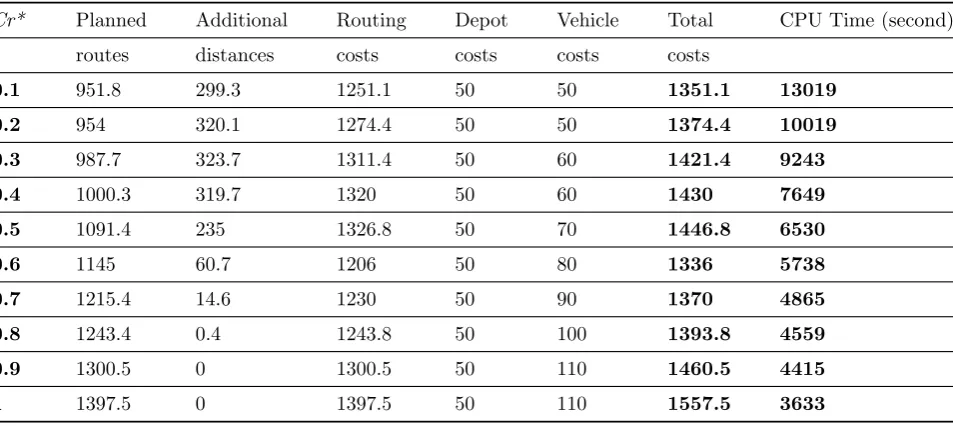
Table 3: The average of results with differentCr∗ when the number of customers is 100.
Cr* Planned Additional Routing Depot Vehicle Total CPU Time (second)
routes distances costs costs costs costs
0.1 951.8 299.3 1251.1 50 50 1351.1 13019
0.2 954 320.1 1274.4 50 50 1374.4 10019
0.3 987.7 323.7 1311.4 50 60 1421.4 9243
0.4 1000.3 319.7 1320 50 60 1430 7649
0.5 1091.4 235 1326.8 50 70 1446.8 6530
0.6 1145 60.7 1206 50 80 1336 5738
0.7 1215.4 14.6 1230 50 90 1370 4865
0.8 1243.4 0.4 1243.8 50 100 1393.8 4559
0.9 1300.5 0 1300.5 50 110 1460.5 4415
1 1397.5 0 1397.5 50 110 1557.5 3633
Ujkt ∈ {N ∪0} ∀j∈J; ∀k∈K; ∀t∈T
(3.20)
The objective function (3.8) represents sum of the fixed depot location costs, fixed costs of em-ploying vehicles, and travel costs, respectively. The objective function (3.9) seeks to minimize total additional travel distance due to routes’
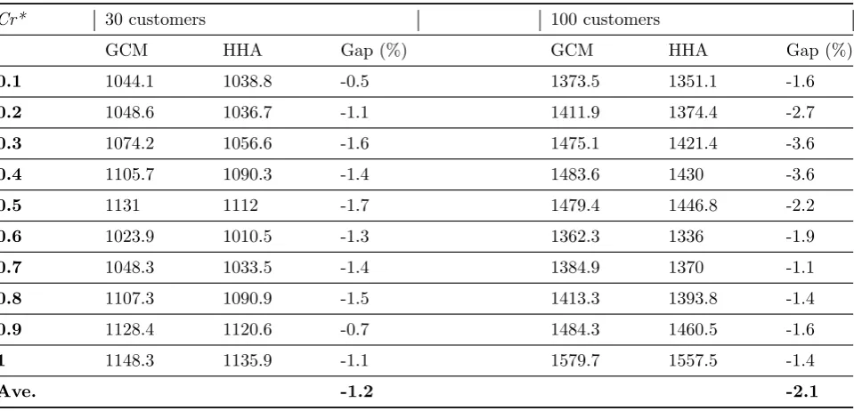
Table 4: Comparison of results between two solving approaches for the CLRP-FD.
Cr* 30 customers 100 customers
GCM HHA Gap (%) GCM HHA Gap (%)
0.1 1044.1 1038.8 -0.5 1373.5 1351.1 -1.6
0.2 1048.6 1036.7 -1.1 1411.9 1374.4 -2.7
0.3 1074.2 1056.6 -1.6 1475.1 1421.4 -3.6
0.4 1105.7 1090.3 -1.4 1483.6 1430 -3.6
0.5 1131 1112 -1.7 1479.4 1446.8 -2.2
0.6 1023.9 1010.5 -1.3 1362.3 1336 -1.9
0.7 1048.3 1033.5 -1.4 1384.9 1370 -1.1
0.8 1107.3 1090.9 -1.5 1413.3 1393.8 -1.4
0.9 1128.4 1120.6 -0.7 1484.3 1460.5 -1.6
1 1148.3 1135.9 -1.1 1579.7 1557.5 -1.4
Ave. -1.2 -2.1
Table 5: The summarized results of two test instances with their lower bounds.
Quality of solutions CPU Time (second)
Instance HHA solution Lower bound Gap (%) HHA solution Lower bound Gap (%)
30 customers 1010.5 620.4 62.9 477 420 13.6
100 customers 1336 969 37.9 5738 2980 25.8
Table 6: The summarized results of LINGO 11 on lower bounds.
Lower bound CPU Time (second)
Instance HHA Lingo 11 Gap (%) HHA Lingo 11 Gap (%)
30 customers 620.4 728 17.3 420 2880 585.7
100 customers 969 infeasible - 4560 28800 531.6
respectively. Each customer should be served within one route only and the customers should have only one predecessor, which is stated by constraint (3.12). The sub-tour elimination con-straints are assured in (3.13). The continuity of the routes and return to the original depot are guaranteed through constraints (3.14) and (3.15). Constraints (3.16) ensure that a customer must be assigned to a depot if there is a route connect-ing them. Constraints (3.17), (3.18), and (3.19) specify the binary variables used in the formula-tion and finally, auxiliary variables taking posi-tive values are declared in (3.20).
4
Proposed hybrid heuristic
al-gorithm for the CLRP-FD
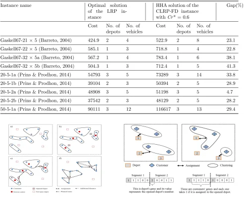
Table 7: Performance of HHA on some CLRP-FD instances obtained from standard test sets of CLRP.
Instance name Optimal solution of the LRP in-stance
HHA solution of the CLRP-FD instance withCr* = 0.6
Gap(%)
Cost No. of No. of Cost No. of No. of depots vehicles depots vehicles
Gaskell67-21×5 (Barreto, 2004) 424.9 2 4 522.9 2 8 23.1
Gaskell67-22×5 (Barreto, 2004) 585.1 1 3 718.8 1 4 22.8
Gaskell67-32×5a (Barreto, 2004) 567.2 1 4 783.4 1 6 38.1
Gaskell67-32×5b (Barreto, 2004) 504.3 1 3 712.4 1 5 41.3
20-5-1a (Prins & Prodhon, 2014) 54793 3 5 73289 3 14 33.8
20-5-1b (Prins & Prodhon, 2014) 39104 2 3 50394 2 5 28.9
20-5-2a (Prins & Prodhon, 2014) 48908 3 5 51198 3 5 4.7
20-5-2b (Prins & Prodhon, 2014) 37542 2 3 48129 2 5 28.2
50-5-1a (Prins & Prodhon, 2014) 90111 3 12 116617 3 13 29.4
Figure 1: Illustrative example of the first phase of the HHA
step, considering the distance between the depot and the gravity center of the clusters as well as the capacity of the depot (Fig. 1(c)). Finally, in the fourth step, ant colony system (ACS) forms an admissible tour among each cluster and relevant depot (Fig. 1(d)). In this step, the stochastic simulation is also used to determine the demand of customers. This helps to evaluate the planned routes and calculate additional distances due to route failures.
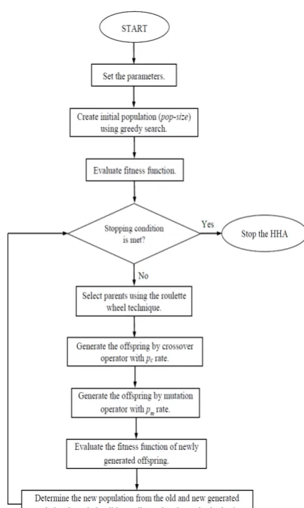
In the second phase of the HHA, a genetic al-gorithm (GA) is used to improve the initial pop-ulation generated through the first phase. In the first step of this phase, a generation of offspring is produced by crossover and mutation operators. Then, the population of solutions is evaluated by using a proper fitness function. In the next step,
Figure 2: Illustration of two instances with chro-mosome representation.
the best solutions are applied to form the next generation of offspring. This improvement pro-cedure will be continued until the termination condition is matched. When a better solution is obtained, the new best solution will be replaced with the past best-known solution. The problem is initialized by defining a plane comprising the set of depots, M, customers, N, and their coor-dinate points. Details of the HHA’s phases are described in following sub-sections.
4.1 Creating the initial population
Figure 3: Crossover operator employed in the customers’ genes of each segment
Figure 4: Mutation operator employed in the sec-tion of the depots’ genes.
the obtained solutions are considered as an ini-tial population of GA to be applied in the second phase. First phase includes four steps as follows:
4.1.1 Clustering the customers
The first step for creating the initial population in GCM is clustering the customers. The customers are grouped considering their distances and their fuzzy demands in addition to the capacity of the vehicles. A greedy search algorithm is used to select a set of customers. At first, to form a clus-ter, a customer is selected randomly from a set of non-clustered customers belongs to N. The al-gorithm searches for the closest customer to the last added customer of the current cluster. Note that, the greedy selection of the next customer may cause a shorter tour and then lower routing costs. The closest customer is not assigned to the cluster if its demand exceeds the remaining ca-pacity of the vehicle, considering the dispatcher preference index value and the credibility of the customer. When a new customer is selected to be assigned to a cluster, total fuzzy demand of
Figure 5: Flowchart of the hybrid heuristic algo-rithm (HHA).
current members of the cluster is calculated and compared to the capacity of the vehicle. If the re-lationCr =Cr∗ is fulfilled (according to the for-mulation (3.5)), then the new customer is allowed to assign to the current cluster. Otherwise, last selected customer is withdrawn from the cluster. The greedy search algorithm seeks for a new cus-tomer close to the last added member of the clus-ter among the ungrouped customers. This proce-dure helps to use the maximum capacity of vehi-cles. The algorithm forms a new cluster if there is no customer to be assigned to current cluster considering the capacity of vehicles and fuzzy de-mand of customers. When there is no unassigned customer, the process of clustering stops.
4.1.2 Establishing the depot(s)
Figure 6: The changes of costs with different of Cr∗ when the number of customers is 30.
Figure 7: The changes of costs with different of Cr∗ when the number of customers is 100.
equation (4.21), in which (x(C),y(C)) is the coor-dinates of the gravity center of clusterC, (xj,yj)
is the coordinates of customer j, and nC is the
number of customers assigned to clusterC.
(
x(C), y(C)
)
=
(∑ j∈Cxj
nC
,
∑ j∈Cyj
nC )
(4.21)
Secondly, the sum of distances of each poten-tial site from all gravity centers of the clusters is calculated. The potential sites are sorted in an ascending order and ranked from 1 to M ac-cording to their Euclidean distance from the grav-ity centers of clusters. The Euclidean distance is calculated by equation (4.22). In this equation, (x∗,y∗) is the coordinates of the desired potential site among all potential sites. Moreover, wi is
the total Euclidean distance of the potential site
j from all gravity centers of the clusters, (xi,yi) is
the coordinates of the potential sitei, (x(C),y(C)) is the coordinates of the gravity center of cluster
C, m is the number of clusters, and M is the
number of potential sites.
(x∗, y∗) : M ininmize wi
=
m ∑
C=1
[
(xi−x(C))2+ (yi−y(C))2
]1/ 2
∀i= 1, ..., M (4.22)
The top-ranked potential site is selected to be established. As it will be mentioned in next step, if the capacity of the current opened depot is un-able to fulfill all clusters considering total demand of each cluster and theCr∗∗value, the next poten-tial site in the sorted list is selected to serve the remaining clusters. This procedure (i.e., estab-lishing the depot(s)) is repeated until all clusters can be served.
4.1.3 Allocating clusters to depots
In third step of GCM, the clusters are respec-tively allocated to the ranked depots. Each de-pot serves clusters as many as possible, based on the value ofCr∗∗and the credibility that the next cluster demand does not exceed the remaining ca-pacity of the depot. To allocate the clusters, the Euclidian distance of the gravity center of each cluster to the top-ranked depot is calculated. Af-terwards, the clusters are ranked in an ascend-ing order based on the distance of their gravity centers to the top-ranked depot. The top-ranked cluster is allocated to the top-ranked depot, if the relation Cr = Cr∗∗ is fulfilled. If there is an empty capacity for the top-ranked depot, the second-ranked cluster is allocated to the depot considering the above relation. The allocation of clusters to the top-ranked depot is finished when there is not enough capacity to serve another clus-ter. In this situation, the allocation procedure is repeated for next-ranked depots until all clusters are allocated.
4.1.4 Routing
pheromone of shorter route increases and there-fore, more ants move along that way. Artificial ants construct a solution by selecting a customer to visit sequentially until all customers are vis-ited. In fact, ants select the next customer to visit using a combination of heuristic and pheromone information. A local updating rule is applied to modify the pheromone on the selected route, dur-ing the construction of a route. When all ants construct their tours, the amount of pheromone of the best selected route and the global best so-lution, are updated according to the global up-dating rule. More details on ACS can be found in [7,49,17].
As mentioned before, in this paper the demand of each customer is a triangular fuzzy number, so it cannot be directly considered as a deterministic number like other methods that tackle the deter-ministic CLRP. Since the real value of demand is identified as the vehicle reaches the customer, the simulation experiment is used to estimate the deterministic value of each customer’s demand. For each feasible planned route that the solution of the HHA stands for, additional distances (fk)
due to route failures are obtained by a stochas-tic simulation algorithm. The steps of stochasstochas-tic simulation are summarized as follows:
Step 1: Estimate the “actual” demand of each customer by following processes: (2.1) randomly generate a real numberD in the interval between the left and right bounds of the triangular fuzzy demand of the customer, and compute its mem-bership m; (2.2) generate a random number r in the interval of [0,1]; (2.3) compare r and m, if r
= m, then “actual” demand of the customer is adopted to D; otherwise, it is not accepted that the demand of the customer is considered D. In this case, random numbersD andr are generated repeatedly until random numbers D and r are found such that relation r =m is satisfied; (3.4) check and repeat (2.1) till (2.3), and terminate the process when each customer has a simulated “actual” demand quantity.
Step 2: Move vehicles along the routes de-signed using credibility theory. Apply ACS to the routes and calculate the additional distance due to route failures in terms of “actual” demand. Step 3: Repeat Steps 1 and 2 M times. In this work, the proper value ofM was considered 300 after some computational experiments.
Step 4: Compute the average additional
dis-tances that come out of stochastic simulation, and return it as the additional distance (fk).
Note that, the routing cost in the CLRP-FD, denoted by f(S) in which S is a solution among
pop-size solutions, consists of two parts: ad-ditional distances and planned route distances. The additional distances are calculated by the stochastic simulation. Instead, prior to calculat-ing the additional distance the planned route dis-tances between the depots and allocated clusters are computed by ACS without considering the fuzzy demands of customers.
4.2 Improving the solutions
In the second phase of the HHA, a genetic algo-rithm (GA), firstly introduced by Holland [21], is used to improve the solutions that come out of the first phase. As mentioned before, the CLRP belongs to the class of NP-hard problems. For this reason, the exact solution methods become highly time-consuming as the problem instances increase in size. Therefore, due to the combina-torial nature of the CLRP-FD and the efficiency of population-based algorithms in solving combi-natorial problems, GA is applied to improve the initial solutions. In fact, the main motivation for this selection is that in recent years, a large num-ber of GAs have developed by researchers with considerable success in solving routing-like prob-lems [18,19,20,51].
The idea behind a GA is to model the natural evolution by using genetic inheritance together with Darwin’s theory. A population of individu-als representing tentative solutions is maintained over many generations. New individuals are pro-duced by combining members of the population via crossover and mutation operators, and then replace existing individuals based on their fitness functions [35].
and mutation methods are shown by an exam-ple. Finally, the evaluation process to produce the next generation is described.
4.2.1 Chromosome representation
The GA requires a string representation scheme (chromosome) to encode solutions of the prob-lem. In this work, each chromosome consists of several segments directly related to the number of clusters. Moreover, each segment is a string of binary values. An example of solution obtained from the first phase along with its encoded chro-mosome is shown in Fig. 2. Each segment of the chromosome is made up of some genes such that it displays the opened depot and the customers who assigned to the depot. The value of the first gene of a segment represents the depot’s num-ber (integers between 1 andM). The position of other genes of a segment represents customers’ numbers in which binary value of each gene de-termines whether the customer assigned to the depot or not.
4.2.2 Selection operator
The selection operation is a process to select two individuals from the current population. In this study, the roulette wheel selection procedure is employed in such a way that the selection prob-ability of each chromosome is proportional to its fitness value. Moreover, based on the fitness val-ues, a tentative set of solutions (selected among current population) is stored and passed directly to the new population for elite protection. Other chromosomes of the new population are gener-ated through an evolutionary loop applying the crossover and mutation operators. More pre-cisely, the selection probability of chromosome
S denoted by pselection(S) is expressed by Eq.
(4.23) in which f it(S) is the fitness of chromo-someS. Recall that, S is a given solution among
pop-size solutions obtained from first phase of HHA.
pselection(S) =
f it(S)
∑pop−size S=1 f it(S)
(4.23)
Fitness of chromosomeS is defined by Eq. (4.24) as follows:
f it(S) = 1
f(S) (4.24)
In whichf(S) is routing cost associated with the solutionS. Since, the routing cost should be min-imized, the inverse of routing cost of a solution is considered as fitness value. Meanwhile, the value off(S) for each solution is obtained by the method explained in section 4.1.4.
4.2.3 Crossover operator
In the proposed GA, crossover operator is only used in the customers’ genes. To do so, a ran-dom number, say n, is generated based on a dis-crete uniform distribution in {1,2,3, . . . , N}. In the crossover operator, in children, the content of the customers’ genes until n will remain the same as the first parent. The genes from n+1 toN are filled by the order that remaining genes appear in the second parent. This work continues for remaining segments of the chromosome while the crossover point is fixed. In this step, regard-ing the crossover rate, say pc, the new solutions
(offspring) are generated. Fig. 3 exemplifies the crossover operator applied in the second phase.
4.2.4 Mutation operator
To make the search more diversified and to escape from local optima, mutation operator is used on the depots’ genes. To do so, a random number, say m, is generated based on a discrete uniform distribution in{1, 2, 3, . . . ,M}. In the mutation operator, in children, the content of the depot’s gene takes the value of m. Note that, the mu-tation of depots’ genes on remaining segments of the chromosome can be changed by selecting an-other random number in{1, 2, 3, . . . ,M}. Fig. 4
shows a swap mutation done at the depots’ gene of each segment. In this step, pm is considered as
mutation rate such that new mutated solutions (offspring) are generated based on this value.
4.2.5 Reproduction
generation is selected from among the old gen-eration and the new generated offspring. Two mechanisms, namely elitism policy and roulette wheel selection, are used in the proposed algo-rithm to select the new generation. Indeed, the former empowers the intensification capability of the algorithm, and the latter enhances its diver-sification. To build the new generation, a pre-determined percentage, say pe, of the
chromo-somes are selected based on the elitism policy and the roulette wheel selection technique is used to select the rest. It is notable that after some com-putational experiments, the proper values of pc,
pmandpewere considered 0.8, 0.2 and 0.6,
respec-tively. The general structure of the HHA is given by Fig. 5.
5
Computational results
5.1 Sensitivity analysis of the parame-ters of the model CLRP-FD
In this section, some numerical experiments are given to show the performance of the CLRP-FD’s model and the efficiency of the HHA. In the first experiment, to evaluate the sensitivity of the pa-rameters of the model, different size of instances is considered to conduct computational experi-ments. It is assumed that there are 30 customers and 5 candidate depots for a small-size instance, and 100 customers and 7 candidate depots for a large-size instance. In each instance, the co-ordinates of all customers and depots are gen-erated randomly in [100×100]. Moreover, the fuzzy demands of customers, which are triangu-lar fuzzy numbers like ˜d = (d1, d2, d3), are se-lected randomly. More precisely,d1,d2andd3are randomly generated within [10,35], [36,60] and [61,110], respectively. The relative data for two test instances are listed in Table1. Note that, the generated test instances are similar to the real-world cases and entirely consistent with the real data. Thus, the obtained results can be applied for real-world application.
The HHA is coded in MATLAB 7.10.0 on a com-puter, holding Intel CoreT M Duo CPU T2450 2.00 GHz. To find the proper value of dispatcher preference index (Cr*), its value is changed in the interval of 0.1 to 1 by a step of 0.1. In this work, the value of assignment preference index (Cr∗∗) is set to 1 due to convenience and reducing the num-ber of different investigative statues. The average
computational results of 10 times are given in Ta-bles2and3for small and large-size instances, re-spectively. The columns of the tables respectively labeled: the dispatcher preference index denoted byCr∗, the cost of planned routes, the cost of ad-ditional distances, routing cost that include the planned routes and additional distances, depot cost, vehicle cost, total cost that consist of rout-ing cost as well as depot and vehicle’s costs and finally, the CPU time of solutions. For more con-venience, summary of the results are depicted in Figs. 6 and 7. As it is shown in Tables 2-3 and also in Figs. 6-7, when the value of dispatcher preference index equals 0.6, the total cost has its own minimum value.
According to Figs. 6 and 7, lower values of pa-rameter Cr∗ denote a tendency to use total ve-hicle capacity. These values are associated with the routes with the shorter planned distances. On the other hand, lower values of parameterCr∗ in-crease the number of cases in which vehicles visit customers but are unable to serve them, thereby lead to increase the total additional distance due to the “failure”. Higher values of parameter Cr∗
are characterized by less utilization of vehicle ca-pacity along the planned routes and fewer addi-tional distances. Therefore, the proper value of
Cr∗ is approximately around 0.6 based on the to-tal cost.
5.2 Performance of the proposed hy-brid heuristic algorithm
In this section, the efficiency of the HHA is com-pared with the conventional approach developed for solving the CLRP-FD. To evaluate the effi-ciency of the proposed HHA, the results of Ta-bles 2-3are compared with the greedy clustering method (GCM) that is similar to the first phase of the HHA. Table4indicates the summary of com-putations on instances described in section 5.1. First column of the table shows the dispatcher preference index (Cr*). The next three columns along with the last three columns show the com-parison of results between the GCM proposed by Zare Mehrjerdi and Nadizadeh [59] and the HHA developed in this work for small and large-size instances, respectively. Note that, the column la-beled ”Gap” reports the gap percentage that is computed for each instance as 100×[(OFVHHA
– OFVGCM)/ OFVGCM] where OFVHHA and
of HHA and GCM, respectively. As shown in Ta-ble 4, the HHA has improved solutions of two instances for all Cr∗ values. So, the HHA is more efficient than the GCM in terms of solu-tion quality. Further performance assessment of the HHA is the comparison of the results with the lower bound of solutions that obtained from an exact algorithm. A simple method for cre-ating a lower bound is through the relaxation of some assumptions that the problem is based on or the constraint(s) used in modeling the problem. To obtain the lower bound of CLRP-FD, the as-sumption of fuzzy demand of customers is ignored and the demand of each customer is set to its left boundary. In other words, the problem of CLRP-FD changes to CLRP in such a way that the left boundary of the triangular fuzzy demand is con-sidered as the demand of each customer (i.e.,d1j
instead of ˜dj = (d1j, d2j, d3j)). To do so, the
constraints (3.10) in the model changes as follows:
∑
i∈V ∑
j∈J
d1jxijk≤Q ∀ k∈K (5.25)
Clearly, when the left boundary of fuzzy mands are considered as the deterministic de-mands of customers, the total demand of cus-tomers is decreased in compare to a case in which the demands are fuzzy. Moreover, fewer total de-mands result in less utilization of depots and ve-hicles and then less total cost. Thus, considering the d1j as the demand of customer j provides a lower bound for the CLRP-FD’s solution. Tables
5 and 6 show the lower bound of the instances described in section 5.1 as well as a summary of the results in terms of the quality of solutions and the computational solutions times.
Table 5 indicates the lower bound of two in-stances explained in section5.1. The first column of the table is the name of instances and the next three columns summarize the quality of solutions consists of HHA solution, lower bound and the gap between them. Note that, the column named HHA solution is obtained from the total cost of Table2 and 3 with credibility of 0.6, which have the minimum total costs among other credibility values. The gap percentage for each instance is also computed as 100 ×[(HHA solution – Lower bound)/ Lower bound]. Three last columns of the Table5indicate the CPU time of HHA solutions and lower bound and the gap between them. Re-garding the results presented in Table 5, fixing
the demand of all customers to their left bound-aries has significant effects on both quality and CPU time of solutions. As shown in Table 5, if the assumption of the fuzzy demands is omitted, the quality of solutions will be improved by 62.9% and 37.9% for small and large-size instances, re-spectively. Argue is that, the less utilization of vehicles and depots cause the additional distance omission when the customer demand is determin-istic. This is the sort of situation that reduces the lower bound values to 620.4 and 969 for small and large-size instances, respectively. Similarly, if the assumption of fuzzy demand of customers is re-laxed, the average CPU time is reduced by 13.6% and 25.8% for small and large-size instances, re-spectively.
It is of interest to notice that, to obtain the lower bound, commercial solver of LINGO 11 was also applied in addition to the HHA. However, it was unable to solve large-size instance and the solu-tion was infeasible after 8 hours of running time. Table 6 shows the lower bound and CPU time of the instances that solved by both LINGO 11 and HHA. Consequently, as seen in Table 6, the proposed HHA is more efficient in compare to LINGO solver in terms of not only quality of lower bounds, but also CPU times of solutions.
Further results of the numerical experiment for evaluating the efficiency of HHA and the perfor-mance of CLRP-FD’s model is shown in Table
7. Table 7 consists of 9 standard test instances that exist in the literature of CLRP [41]. To use the standard test instances of CLRP in case of CLRP-FD, some changes on CLRP instances are required. The following heuristic steps show the process of changing a CLRP instance to a CLRP-FD one.
Step 1: At first, the determinist demand of each customer transforms to a triangular fuzzy demand as follows: (2.1) consider the determin-istic demand of each customer in the CLRP as the left boundary of fuzzy demand in CLRP-FD; (2.2) calculate the right boundary of fuzzy de-mand by triple the left boundary obtained from (2.1); (2.3) consider a random number in the range of 1.5 to 2.5 times of the left boundary as the middle number of triangular fuzzy demand.
Step 2: Consider the maximum right bound-aries of fuzzy demands of all customers as D3j
(i.e. D3j = max
j∈J{d3j}. CompareD3j with the
Q. If the relation D3j ≤ Qis satisfied, then
con-sider Q as the vehicle capacity of the CLRP-FD instance. Otherwise, consider D3j as the vehicle
capacity of the CLRP-FD instance.
Step 3: Triple the depot’s capacity of the LRP instance and consider that as the depot’s capacity of CLRP-FD instance.
According to above steps, it is clear when the left boundaries of fuzzy demands of CLRP-FD instance are equal with the demands of CLRP instance, the solution of CLRP instance will be as a lower bound for the solution of CLRP-FD instance. Table 7 shows the summary of results on several standard test instances. First column of the table indicates the name of standard test instances on CLRP that can be found in [5,37]. Three next columns show the optimal solutions obtained from the algorithms in the literature of CLRP. The solutions obtained by HHA withCr∗
value of 0.6 are shown at the next three columns. The last column of Table 7 indicates the gap of costs between HHA and optimal solutions. As a result of Table7, it is concluded that the solution of CLRP for each instance is a lower bound for the solution of CLRP-FD.
6
Conclusion
and
future
re-search
Logistics costs often represent a large portion of the expenses of companies. In order to reduce them, facility location and vehicle routing are crucial. In the management decision of the logis-tics, facility location problems and vehicle routing problems are interdependent. But most of time, they are considered separately. This cannot re-duce company’s total cost in reality and will also increase the total cost sometimes. The location-routing problem (LRP) overcomes above draw-back by simultaneously tackling facility location problem and vehicle routing problem. Nowadays, there are many literatures to research LRP, but most of them have only studied the LRPs with deterministic demands. This paper contributes to the capacitated location-routing problem with fuzzy demands that is closer to reality in the real-world. A fuzzy chance-constrained programming formulation has been developed for the problem. To solve the problem, a hybrid heuristic algo-rithm (HHA) with two main phases was proposed
in which greedy search algorithm was applied to generate initial population of solutions at the first phase and genetic algorithm was used for further improvement of the solutions at the second. The additional distances due to fuzzy demands and route failures were estimated by stochastic sim-ulation for each planned route. For performance evaluation of the model and the proposed HHA, different numerical experiments were carried out. The computational experiments have shown that the dispatcher preference index (Cr∗) greatly in-fluences the planned routes’ length, additional distance, and fixed cost of depots and vehicles. So, the best value of this sensitive parameter of the model was obtained via conducting compu-tational experiments. Comparison of the results between HHA and GCM (i.e., the developed al-gorithm in the literature of CLRP-FD) has indi-cated that the HHA is more efficient than GCM. Moreover, the lower bound of solutions was com-puted by the HHA and the commercial solver of LINGO 11. Finally, numerical experiments with standard test instances of CLRP have carried out to show the performance of the CLRP-FD’s model.
This paper has some limitation that is capable for future researches: (a) investigating the effect of another major parameter of the model, named assignment preference index (Cr∗∗), on the length of the planned routes and the additional distances traveled by vehicles due to route failures by statis-tical methods like design of experiments, (b) con-sidering the CLRP-FD with pickup and delivery, (c) given the demand of customers as trapezoidal fuzzy instead of triangular fuzzy, (d) developing other solution algorithms, e.g. hybrid evolution-ary algorithms, (e) proposing new stochastic sim-ulation for estimating both actual demand of cus-tomers and additional distances, and (f) develop-ing the model under more realistic assumptions, e.g. heterogeneous fleet.
References
[1] M. Albareda-Sambola, J. A Diaz, E. Fernan-dez, Computers & Operations Research, 32, 407-428 (2005).
[3] S. Balin, Information Sciences, 181, 3551-3569 (2011).
[4] S. Barreto, C. Ferreira, J. Paixao, B. Sousa Santos,European Journal of Operational Re-search, 179, 968-977 (2007).
[5] S. Barreto, An´alise e Modeliza¸c˜ao de Prob-lemas de localiza¸c˜ao-distribui¸c˜ao (2004).
[6] J. M. Belenguer, E. Benavent, C. Prins, C. Prodhon, R. Wolfler-Calvo, Computers & Operations Research, 38, 931-941 (2011).
[7] L. Bouhafs, A. Hajjam, A. Koukam,Lecture Notes in Computer Science, 4251, 409-416 (2006).
[8] L. Bouhafs, A. Hajjam, A. Koukam,Journal of Artificial Intelligence: Theory and Appli-cation, 1, 31-34 (2010).
[9] C. Contardo, V. Hemmelmayr, T. G. Crainic, Computers & Operations Research, 39, 3185-3199 (2012).
[10] H. Derbel, B. Jarboui, S. Hanafi, H. Chab-choub,Expert Systems with Applications, 39, 2865-2871 (2012).
[11] M. Dorigo, L. M. Gambardella, PPSN springer-Verlag Berlin, 656-665 (1996). [12] M. Drexl, M. Schneider,European Journal of
Operational Research, 241, 283-308 (2015). [13] C. Duhamel, P. Lacomme, C. Prins, C.
Prod-hon,Computers & Operations Research, 37, 1912-1923 (2010).
[14] C. Erbao, L. Mingyong, Journal of Compu-tational and Applied Mathematics, 231, 302-310 (2009).
[15] C. Erbao, L. Mingyong,Expert Systems with Applications, 37, 2405-2411 (2010).
[16] M. H. Fazel Zarandi, A. Hemmati, S. Davari, B. Turksen, Knowledge-Based Systems, 37, 480-489 (2013).
[17] S. Gao, Y. Wang, J. Cheng, Y. Inazumi, Z. Tang, Applied Mathematics and Computa-tion, 285, 149-173 (2016).
[18] M. Gen, A. Syarif, Computers & Industrial Engineering, 48, 799-809 (2005).
[19] K. Ghoseiri, S. F. Ghannadpour, Applied Soft Computing, 10, 1096-1107 (2010). [20] W. Ho, G. T. Ho, P. Ji, H. C. Lau,
Engineer-ing Applications of Artificial Intelligence, 21, 548-557 (2008).
[21] J. H. Holland,U Michigan Press, (1975).s [22] I. Karaoglan, F. Altiparmak, I. Kara, B.
Dengiz, European Journal of Operational Research, 211, 318-332 (2011).
[23] I. Karaoglan, F. Altiparmak, I. Kara, B. Dengiz, Omega, 40, 465-477 (2012).
[24] A. Kaufmann, Introduction to the theory of fuzzy subsets, Vol. I. (1975).
[25] Y. F. Lan, Y. K. Liu, G. J. Sun, Journal of Computational and Applied Mathematics, 231, 208-221 (2009).
[26] S. R. Li, B. B. Keskin, Journal of the Op-erational Research Society, 65, 1711-1725 (2013).
[27] C. K. Y. Lin, C. K. Chow, A. Chen, Com-puters & Industrial Engineering, 43, 5-25 (2002).
[28] B. Liu, Uncertain Theory: An introduce to its axiomatic foundations, (2004).
[29] S. M. H. Manzour-al-Ajdad, S. A. Torabi, S. Salhi,Computers & Operations Research, 39, 461-470 (2012).
[30] Y. Marinakis, M. Marinaki, Journal of Mathematical Modelling and Algorithms, 7, 59-78 (2008).
[31] A. Nadizadeh, H. Hosseini Nasab, European Journal of Operational Research, 238, 458-470 (2014).
[32] A. Nadizadeh, R. Sahraeian, A. Sabzevari Zadeh, S. M. Homayouni,African Journal of Business Management, 5, 7499-7506 (2011). [33] G. Nagy, S. Salhi,Journal of the Operational
Research Society, 47, 1166-1174 (1996). [34] G. Nagy, S. Salhi, European Journal of
Op-erational Research, 177, 649-672, (2007). [35] H. Nazif, L. S. Lee, Applied Mathematical
[36] V. P. Nguyen, C. Prins, C. Prodhon, Euro-pean Journal of Operational Research, 216, 113-126 (2012).
[37] C. Prins, C.Prodhon,Nouveaux algorithmes pour le probl`eme de localisationet routage sous contraintes de capacit´e, (2004).
[38] C. Prins, C. Prodhon, R. Wolfler Calvo,
4OR, 4, 221-238 (2006a).
[39] C. Prins, C. Prodhon, R. Wolfler Calvo, Lec-ture Notes in Computer Science, 3906, 183-194 (2006b).
[40] C. Prins, C. Prodhon, R. Wolfler Calvo,
Transportation Science, 41, 470-483 (2007).
[41] C. Prodhon, http://prodhonc.free.fr/ Instances/instances_us.htm/(2008). [42] C. Prodhon, European Journal of
Opera-tional Research, 210, 204-212 (2011).
[43] C. Prodhon, C. Prins, European Journal of Operational Research, 238, 1-17 (2014).
[44] S. Salhi, G.K. Rand, European Journal of Operational Research, 39, 150-156 (1989).
[45] K. Sheriff, S. Nachiappan, H. Min, Journal of the Operational Research Society, 65, 873-887 (1989).
[46] R. Srivastava,Omega, 21, 497-506 (1993).
[47] A. Stenger, M. Schneider, M. Schwind, D. Vigo, International journal of production economics, 140, 702-712 (2012).
[48] C. J. Ting, C. H. Chen,International journal of production economics, 141, 34-44 (2013).
[49] C. W. Tsai, S. P. Tseng, C. S. Yang, M. C. Chiang, Applied Soft Computing, 13, 3008-3020 (2013).
[50] D. Tuzun, L. I. Burke, European Journal of Operational Research, 116, 87-99 (1999).
[51] Z. Ursani, D. Essam, D. Cornforth, R. Stocker, Applied Soft Computing, 11, 5375-5390 (2011).
[52] X. Wang, X. Sun, Y. Fang,2005 IEEE Inter-national Conference on Systems, Man and Cybernetics, 4, 3338-3343 (2005).
[53] T. H. Wu, C. Low, J. W. Bai,Computers & Operations Research, 29, 1393-1415 (2002).
[54] V. F. Yu, S. W. Lin, W. Lee, Computers & Industrial Engineering, 58, 288-299 (2010).
[55] L. A. Zadeh, Information and Control, 8, 338-353 (1965).
[56] L.A. Zadeh, Fuzzy Sets and Systems, 1, 3-28 (1978).
[57] M. Zarandi, A. Hemmati, S. Davari, I. Turk-sen, Knowledge-Based Systems, 37, 480-489 (2013).
[58] M. H. F. Zarandi, A. Hemmati, S. Davari,
Expert Systems with Applications, 38, 10075-10084 (2011).
[59] Y. Zare Mehrjerdi, A. Nadizadeh, European Journal of Operational Research, 229, 75-84 (2013).
[60] Y. Zare Mehrjerdi, A. Nadizadeh, Interna-tional Journal of Industrial Engineering & Production Research, 27, 1-19 (2016).
Ali Nadizadeh is Ph.D of Indus-trial engineering. He is group man-ager of Industrial engineering in Ardakan University of Iran. His re-search interests include operation research, combinatorial optimiza-tion and supply chain management issues.