Volume 59, 2019, Pages 1–17
Proceedings of Pragmatics of SAT 2015 and 2018
Evaluating CDCL Restart Schemes
Armin Biere and Andreas Fr¨
ohlich
Institute for Formal Models and Verification Johannes Kepler University, Linz, Austria∗
Abstract
Modern CDCL (conflict-driven clause learning) SAT solvers are used for many practical applications. One of the key ingredients of state-of-the-art CDCL solvers are efficient restart schemes. The main contribution of this work is an extensive empirical evaluation of various restart strategies. We show that optimal static restart intervals are not only correlated with the satisfiability status of a certain instance, but also with the more specific problem class of the given benchmark. We further compare uniform restart intervals with the performance of non-uniform restart schemes, such as Luby restarts. Finally, we revisit the dynamic restart strategy used in Glucose and propose a new variant thereof, which is based on the concept of exponential moving averages. The resulting implementation in Lingeling improves state-of-the-art performance in SAT solving.
1
Introduction
On application benchmarks,conflict-driven clause learning (CDCL) [22] solvers are considered to be the state-of-the-art in SAT solving and, e.g., the application track of SAT competitions [4,
5] is dominated by CDCL solvers.
Beside learning [23], the most important features of these solvers are dynamic decision heuristics, such as thevariable state independent decaying sum (VSIDS) decision heuristic [24] or variants thereof [6], as well as efficient restart schemes [15, 6,27,2]. In this paper, we focus on the latter. For related work on evaluating CDCL variable scoring schemes, see [9,20].
While earlier restart schemes either used larger intervals or focused on alternating between intervals of different length [15], the particular benefit of frequent restarts has dominated with the introduction of phase saving [26], and has further been improved by reusing (parts of) the trail [28]. Nevertheless, frequent restarts come at an additional cost and, thus, techniques for dynamic restarts often are particularly effective [6,27,2]. In Glucose, for example, restarts are performed whenever the importance of the latest learned clauses appears to be smaller than the average contribution [1,2].
Further, it turned out that frequent restarts are particularly important for unsatisfiable instances, whereas restarting can actually even be harmful for satisfiable ones in many cases [2]. This can be improved by blocking restarts if the current search seems to be close to a solution, e.g., whenever a relatively large fraction of the variables is assigned [2]. Other options are
to use agility as a heuristic for delaying restarts [6], or perform local restarts [27], which are triggered if too many conflicts occurr along a branch. In general, the idea of dynamic restarts for DPLL [11] has already been proposed in [18].
In this paper, we analyze different restart schemes in more detail. We first evaluate restart schemes with fixed intervals on different classes of benchmarks. It is well-known that runtime distributions of satisfiable and unsatisfiable instances differ significantly [13]. While earlier work already discussed the general influence of restart intervals related to the satisfiabilty of an in-stance [2], the effect of restarts on particular classes of instances from the SAT competition [5] has not been analyzed before. We show that, even among satisfiable (SAT) and unsatisfiable (UNSAT) instances, there are classes of benchmarks (buckets) that profit from shorter and longer restart intervals, respectively. Furthermore, with new benchmarks and the steady de-velopment of SAT solvers, it is not clear whether evaluations, such as done in [15], still apply to current state-of-the-art solvers. For example, we show that solvers with fixed size restart intervals can actually perform equally well to those based on the Luby series [21]. A similar conjecture is given in [2], pointing out that the original role of restarts in DPLL based solvers as, e.g., discussed in [14], has changed with the introduction of clause learning.
We also revisit Glucose restarts and discuss their effect compared to static restart intervals. Whereas the original implementation of the Glucose restart scheme requires to keep track of certain values by using a queue, we propose a new variant that does not need additional data structures but, instead, uses the concept ofexponential moving averages. An additional advantage of this technique is the fact that a stronger influence is naturally given to more recent activities. We show that, beside simpler implementation, this further increases the performance of our implementation in Lingeling [8].
The rest of the paper is structured as follows. In Section 2, we first introduce the ex-perimental setup used throughout our paper. We then evaluate static restart strategies in Section3, analyzing the correlation of optimal interval size with particular benchmark classes in Section3.1, as well as strategies with non-uniform intervals in Section 3.2. Afterwards, in Section4, we discuss dynamic restart strategies. We first describe the original Glucose restart scheme in Section4.1and then introduce a modified version by using the concept of exponential moving averages in Section4.2. We also provide details on our implementation in Lingeling in Section4.3. Finally, we conclude in Section5.
2
Experimental Setup
The largest part of our work consists of a substantial empirical evaluation, giving various experimental results, distributed throughout the whole paper, and each used to motivate follow-up discussion. In this section, we therefore want to introduce the experimental setfollow-up used at different places throughout the remaining part of the paper.
All experiments were performed on our benchmark cluster, consisting of 30 nodes with Intel Q9550 Core 2 Quad CPUs running at 2.83GHz and 8 GB of main memory. Each job, e.g., pair of solver (configuration) and benchmark, had exclusive access to one node and CPU, respectively. The time limit was set to 1000 seconds, which is substantially smaller than the original competition time-out of 5000 seconds (competition hardware was further roughly 1.2 times faster). As memory limit, we used 7GB.
As solvers, we used variants of Lingeling that evolved from the SAT competition 2014 version ayv [8] (sc14ayv)1 and Glucose version 4.0 (glu), with small modifications. In the
SAT competition 2014, sc14ayv solved the largest number of instances in the SAT+UNSAT application track. This success of Lingeling can be contributed to the rather long time limit of 5000 seconds as used in the competition. For shorter time limits, Glucose version 2.3 [1,3] from 2013 and particularly its 2014 derivative SWDiA5BY A26 [25] show much better performance, despite lacking many effective preprocessing and inprocessing techniques [16].
Our post competition analysis, see also [9], showed that this effect can be contributed to two different aspects. On the one hand, the benchmark selection scheme used in the SAT competition 2014 (and already in 2013) had a strong influence on those results. Benchmarks were selected in such a way to level out performance of solvers. The goal of the organizers was to make the competition as interesting as possible, with the unfortunate effect, however, that unique solving capabilities, such as inprocessing [16], are deemphasized. On the other hand, our analysis showed that there is indeed an algorithmic feature implemented in all the Glucose variants taking part in the competition, which on these competition benchmarks is quite effective: the Glucose restart strategy [2]. Analyzing and understanding the latter is part of our motivation for this work. Details on the Glucose restart strategy will be given in Section4.1.
To allow a clear comparison, we therefore implemented all techniques used in Glucose 2.3 and SWDiA5BY A26 which were not available in Lingeling, previously. Beside incorporating effective techniques from Glucose and SWDiA5BY, the base line version ba2 of Lingeling, as used in this evaluation, differs from the 2014 version sc14ayv mainly in small pre-processing techniques. Further,reusing the trail [28] andagility [6] are switched off in version ba2, since Glucose 2.3 does not use these features either, and since combining several different heuristics for blocking restarts would conflict with the goal of a clean evaluation of the particular effects. These modifications allow to solve several unsatisfiable combinational hardware equivalence checking “miter” benchmarks [10], submitted 2013. Some of those are solved by our new ba2
version of Lingeling during the first preprocessing phase, without any search. Several others can now be solved because agility was sometimes harmful for those benchmarks. The latter effect, however, might again be partially contributed to the benchmark selection.
Another difference to sc14ayv is the initialization of variable phases. In version ba2, all phases are now initially set to false, as it is also done in Glucose 2.3. This alone allows to solve 13 satisfiable “argumentation” instances [29], submitted 2014, with name prefix “complete. . .”. These 13 instances have a simple solution, with all variables set to false. In contrast, if this is not detected and a more sophisticated phase initialization heuristic like Jeroslow-Wang [17] is triggered before switching to phase saving [26], they become very hard.
For all experiments, we use the 300 instances of the SAT+UNSAT application track of the SAT competition 2014 [5]. With one of our goals being to analyze the correlation between certain benchmark set and the optimal restart strategy of a SAT solver, we split the whole instance set intobuckets. We use the same partitioning as the one suggested by the competition organziers [5], which groups the 300 instances into the following 23 buckets, each containing between 1 and 30 instances (in parenthesis): 2d-strip-packing (4), argumentation (20), bio (11), crypto-aes (8), crypto-des (7), crypto-gos (9), crypto-md5 (21), crypto-sha (29), crypto-vpmc (4), diagnosis (28), fpga-routing (1), hardware-bmc (4), hardware-bmc-ibm (18), hardware-cec (30), hardware-manolios (6), hardware-velev (27), planning (19), scheduling (30), scheduling-pesp (3), software-bit-verif (9), software-bmc (6), symbolic-simulation (1), termination (5).
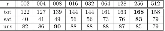
r 002 004 008 016 032 064 128 256 512
tot 122 127 139 144 144 161 163 168 158
sat 40 41 49 56 56 73 76 83 79
uns 82 86 90 88 88 88 87 85 79
Table 1: static-r, number of solved instances on the full SAT competition 2014 benchmark set. The overall results (tot) are also split into SAT (sat) and UNSAT (uns).
3
Static Restarts
In this section, we consider static restarts, i.e., we perform a restart exactly after a certain numberrof conflicts has occured since the last restart. In this context, we distinguish between
r being given as a fixed constant andr being a function of the number of restarts that have already been performed. The first setting results in uniform restart intervals, the latter one can be realized, e.g., by implementing a geometric policy [12,6], or based on the Luby series [21,15].
3.1
Uniform Restart Intervals
We implemented a simple uniform restart strategy in Lingeling, resulting in the solver versions
static-r, with r = 2k for k ∈ {1, . . . ,9}. Obviously, solvers with small r perform frequent
restarts and, therefore, many restarts in total, whereas solvers with largerperform less frequent restarts and, therefore, fewer restarts in total. Table1 summarizes the results we obtained for all differentr on the full benchmark set.
We can see that the version with r = 256 solves the largest number of instances in total. Even more, the number of solved instances is increasing steadily with growingr, up tor= 256. Therefore, largerr seem to perform better, in general. However, Table 1 also shows that the largest number of unsatisfiable instances is actually solved forr= 8, and that this number is decreasing for growing r. This general trend has been observed before. In particular, it has been conjectured that the optimal number of restarts is correlated with the satisfiability status of a given instance [13,2].
Note that this is a very rough classification. For example, it is not clear whether the different versions actually solve the same set of “easier” problems or if there are instances, e.g., even
r 002 004 008 016 032 064 128 256 512
2d-strip-packing 0/2 0/2 0/2 0/2 0/2 1/2 1/2 1/2 2/2
crypto-sha 0/0 0/0 0/0 0/0 1/0 7/0 11/0 13/0 10/0
hardware-cec 0/22 0/23 0/24 0/22 0/22 0/23 0/22 0/21 0/21
hardware-manolios 0/4 0/5 0/5 0/5 0/6 0/6 0/6 0/6 0/6
hardware-velev 5/9 6/10 8/11 8/12 8/12 8/13 8/12 8/11 8/6
planning 6/3 6/5 7/4 7/4 8/4 9/3 9/4 11/4 10/4
scheduling 1/7 0/7 1/7 4/7 6/7 9/7 9/7 11/7 12/7
● ●
● ●
0 200 400 600 800 1000
0 200 400 600 800 1000
static−008 versus static−256
static−008 static−256 ● ● ● ● ● ● ● ● ● ● ● ● ● ● ● ● ● ● ● ● ● ● ●● ● ● ● ● ● ● ● ● ● ● ● ● ● ● ● ● ● ● ● ● ● ● ● ● ● ● ● ● ● ● ● ● ● ● ● ● ● ● ● ● ● ● ● ● ● ● ● ● ● ● ● ● ● ● ● ● ● ● ● ● ● ●●● ● ● ● ● ● ● ● ● ● ● 2d−strip−packing argumentation bio crypto−aes crypto−des crypto−gos crypto−md5 crypto−sha crypto−vpmc diagnosis fpga−routing hardware−bmc hardware−bmc−ibm hardware−cec hardware−manolios hardware−velev planning scheduling scheduling−pesp software−bit−verif software−bmc symbolic−simulation termination
Figure 1: Comparing static-008andstatic-256. Being worse in general, the version withr= 8 is particularly efficient for several bmc, hardware-cec, and software-bit-verif instances.
among the SAT and UNSAT instances, which actually require more frequent or less frequent restarts, respectively. Further, if different versions solved different instances, the observed effect could just be due to introducing non-determinism in the sense ofrrepresenting a random seed. Figure1and Figure2give more details on the effect of restart intervals by splitting the full set of instances into the buckets presented in the previous section. This allows us to see two different aspects. First, both plots immediately allow us to rule out the seed effect. For most buckets, the runtime between its instances is clearly correlated. Second, there is also a significant correlation between the performance of a solver version on certain buckets and its restart interval sizer.
For example, Figure1shows that the instances only solved bystatic-008and not bystatic-256
(or those, where the latter is significantly slower) are mainly bmc, hardware-cec, and software-bit-verif instances. In contrast, scheduling and crypto-sha benchmarks clearly require a larger
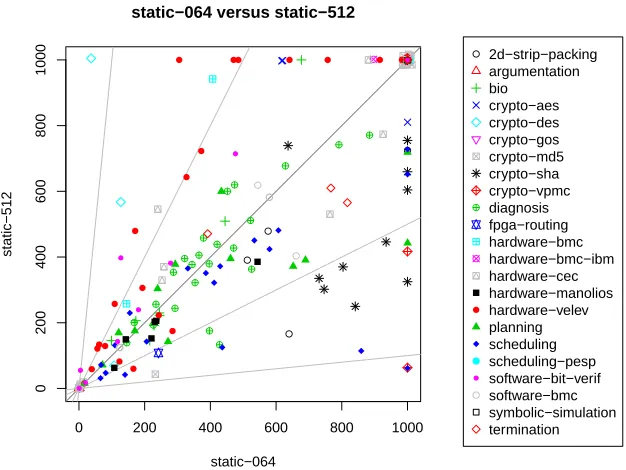
r. Similarly, Figure2 depicts a clear advantage forstatic-064on instances from the hardware-velev bucket. Those seem to require a moderately larger(not as small as 8 but not as large as 512). Most of the scheduling benchmarks are still solved faster with largerr, but the difference in performance is much smaller now. In contrast, crypto-sha instances apear to punish smaller
rmuch stronger while being solved bystatic-512.
● ●
●
●
0 200 400 600 800 1000
0 200 400 600 800 1000
static−064 versus static−512
static−064 static−512 ● ● ● ● ● ● ● ● ● ● ● ● ● ● ● ● ● ● ● ● ● ● ● ● ● ● ● ● ● ● ● ●●●●●●●●●●●●●●● ● ● ● ● ● ● ● ● ● ● ● ● ● ●●●●●●● ● ● ●● ● ● ● ● ● ● ● ● ● ● ● ● ● ● ● ● ● ● ● ● ● ● ● ● ● ● ● ● 2d−strip−packing argumentation bio crypto−aes crypto−des crypto−gos crypto−md5 crypto−sha crypto−vpmc diagnosis fpga−routing hardware−bmc hardware−bmc−ibm hardware−cec hardware−manolios hardware−velev planning scheduling scheduling−pesp software−bit−verif software−bmc symbolic−simulation termination
Figure 2: Comparing static-064 and static-512. With similar overall results (see Table 1), using a moderateris significantly better for hardware-velev instances, whereas crypto-sha and scheduling require a largerr.
hardware-velev bucket do not profit anymore from restart intervals already with r > 8. In most cases, e.g., as for crypto-sha, the maximum number of solved instances is reached for
r= 256, and possibly even decreases afterwards. In contrast, e.g., for scheduling, the number of solved SAT instances increases further withr= 512. The numbers for unsatisfiable instances are less determined. For example, hardware-cec shows the expected behaviour, i.e., versions with smaller restart intervals perform better (with r = 8 being the optimum). However, for hardware-manolios, the trend is reversed, making it profit fromr≥32. In a similar way, more UNSAT instances from the hardware-velev bucket are solved with growingr, up tor= 64 (and performance decreasing afterwards). Actually, for the hardware-velev bucket, using a larger restart interval is more important for the unsatisfiable instances than for the satisfiable ones. Note that the hardware-velev bucket takes another special role in our benchmark set, in the sense that it favours moderate values ofr, while most of the other buckets usually profit most from either low or high values.
luby-b 01 02 04 08 16 32 io-b 001 002 004 008 032 128
tot 156 168 161 163 160 159 161 161 158 153 154 150
sat 72 80 74 77 74 74 80 81 77 74 76 76
uns 84 88 87 86 86 85 81 80 81 79 78 74
avg-r 9 17 31 58 108 203 443 509 601 732 1084 1740
Table 3: luby-bandio-b, number of solved instances on the full SAT competition 2014 benchmark set. Additionally, the average restart interval size (over all instances) is given.
3.2
Non-Uniform Restart Intervals
Non-uniform restart schemes are motivated by two different aspects. First, the optimal size of restart intervals for a given instance is usually not known in advance. Second, a solver might profit from frequent restarts by learning good clauses (e.g., respresenting equivalences, as in the case of “miter” benchmarks) but might still require larger intervals for finding actual solutions. A simple version of non-uniform restart intervals can be realized by using a geometric function. In the most straightforward approach, the size of each different restart interval is just gradually increased. This kind of restart scheme, e.g., has already been used in earlier versions of Minisat [12]. Given theith restart interval, the Minisat scheme defined its length to be 1.5i.
It is easy to see that this function grows very fast and the search is dominated by the largest restart interval, which can contain up to 50% of the total number of conflicts. This leads to very few restarts (logarithmic in the number of conflicts) and, in most cases, this does not represent the desired behaviour. A much better restart scheme is based on the Luby series [21] and was first proposed in [15]. The Luby series is given by 1,1,2,1,1,2,4,1,1,2,1,1,2,4,8, . . ., and the
ith element of the series (i∈N) is formally defined as follows:
luby(i) :=
(
2k−1 ifi= 2k−1
luby(i−2k−1+ 1) if 2k−1≤i <2k−1, for somek∈N.
Note that later versions of Minisat, starting from 2.0, also used a Luby restart policy. Due to the large number of short intervals, the Luby series only grows linearly in the number of restarts, i.e., much slower than the original Minisat scheme. Another interesting property of the Luby series is given by the fact that, assuming we group together all intervals of a specific size r, the sum over all conflicts in each group will be equal (assuming the total number of restarts is 2k−1 for somek∈
N).
static-● ●
● ●
0 200 400 600 800 1000
0 200 400 600 800 1000
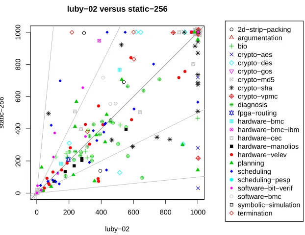
luby−02 versus static−256
luby−02 static−256 ● ● ● ● ● ● ● ● ● ● ● ● ● ● ● ● ● ● ● ● ● ● ● ● ● ● ● ● ● ● ● ● ● ●●●●●●●●●●●●● ● ● ● ● ● ● ● ● ● ● ● ● ● ● ● ● ● ● ● ● ● ● ● ● ● ● ● ● ● ● ● ● ● ● ● ● ● ● ● ● ●● ● ● ● ● ● ● ● ● ● ● 2d−strip−packing argumentation bio crypto−aes crypto−des crypto−gos crypto−md5 crypto−sha crypto−vpmc diagnosis fpga−routing hardware−bmc hardware−bmc−ibm hardware−cec hardware−manolios hardware−velev planning scheduling scheduling−pesp software−bit−verif software−bmc symbolic−simulation termination
Figure 3: Comparing luby-02 and static-256. The performance on individual instances differs significantly. The Luby version, in general, performs better for a broader range of buckets, whereas the uniform version is particularly strong on the crypto-sha bucket.
256. While showing a similar overall performance (see Table1and Table3), the performance on individual instances differs significantly. As already pointed out, a fixed interval size ofr= 256 seems to be particularly beneficial for crypto-sha instances. In contrast, the strongly varying interval size of the Luby strategy allows to improve on a broader range of buckets.
● ●
●
●
0 200 400 600 800 1000
0 200 400 600 800 1000
ema−14 versus static−256
ema−14 static−256 ● ● ● ● ● ● ● ● ● ● ● ● ● ● ● ● ● ● ● ● ● ● ● ● ● ● ● ● ● ● ● ● ● ●●●● ●●●●●●●●● ● ● ● ● ● ● ● ● ● ● ● ● ● ● ● ● ● ● ● ● ● ● ● ● ● ● ● ● ● ● ● ● ● ● ● ● ● ● ● ● ● ● ● ● ● ● ● ● ● ● ● ● 2d−strip−packing argumentation bio crypto−aes crypto−des crypto−gos crypto−md5 crypto−sha crypto−vpmc diagnosis fpga−routing hardware−bmc hardware−bmc−ibm hardware−cec hardware−manolios hardware−velev planning scheduling scheduling−pesp software−bit−verif software−bmc symbolic−simulation termination
Figure 4: Comparingema-14andstatic-256. The version with dynamic restarts (previously not part of Lingeling), based on exponential moving averages, is significantly better.
4
Dynamic Restarts
In the past, most CDCL solvers mainly used static restart schemes, most commonly with non-uniform restart intervals. However, over the last years, certain approaches for dynamic scheduling of restarts have started to play a larger role. For example, PicoSAT [7] first intro-duced the concept ofagility to prohibit restarts under certain restrictions [6] in combination with the inner/outer scheme. Similarly, the latest competition version of Lingeling, sc14ayv, uses a Luby scheme with base interval size 5, and also uses agility to potentially delay restarts. A further dynamic scheme was introduced by Glucose [2], in the following referenced asGlucose restarts. With the better performance of the Glucose restart strategy, agility based approaches are not the focus of this paper. As already pointed out in Section 2, agility is switched off in all our experiments. We also leave comparison with local restarts [27] to future work.
4.1
Glucose Restarts
In Glucose, restarts are based on the literal block distance (LBD) of learned clauses, which is the number of different decision levels in the learned clause [2]. It compares a current “short term average” LBD of learned clauses with a “long term average”. If the short term average is substantially larger than the long term average (say 25%), a restart is triggered, unless a restart happened very recently (less than 50 conflicts earlier). We will make the notion of “average” more precise in the following.
In general, clauses with a small LBD are more important in solving a SAT formula. Due to this, a search in Glucose continues (i.e., no restart takes place) as long as the set of recently learned clauses seems to be “good” according to this measure. Whenever the LBD of recently learned clauses becomes too large, the current search is considered to be less beneficial and, therefore, a restart is performed [2]. We refer to this asforcing a restart.
This dynamic restart strategy already was part of Glucose 1.0. Since this earlier version turned out to be particularly effective for unsatisfiable instances, a further refinement was added in Glucose 2.1. This refinement aimed to improve performance on satisfiable instances [2] as follows. As satisfiable instances sometimes require larger restart intervals, Glucose 2.1 allowed
blocking of restarts. A restart is blocked whenever the solver might be close to finding a satisfying assigment. The concrete policy for blocking restarts is similar to the one for forcing restarts. In particular, the current number of assigned variables is compared with an average of the number of assigned variables over the last 5000 conflicts [2]. This refined version is still part of the most current version of Glucose. As seen from the results of the SAT competition 2014, this dynamic restart strategy turned out to be very effective.
To implement the forcing part of Glucose restarts, two values are needed: The overall average LBD (corresponding to the long term average) and the average LBD over a set of recently learned clauses. Tracking the first one is easy, while calculating the latter one requires a queue of length 50, with 50 being the number of recent clauses to be considered. For blocking restarts, an additional queue of length 5000 is needed [2].
4.2
(Exponential) Moving Averages
We now want to formalize Glucose restarts by introducing the concept of moving averages. In statistics, a moving average is the principle of evaluating a certain window of recent data points related to time series data. It is, e.g., often used in technical analysis of financial data in connection with stock prices. The unweighted mean of the previousw data points is often called asimple moving average(SMA).
Letnbe the index of the current conflict (starting at 1),wbe a window size (e.g., the size of the queue in Glucose), and let ti donate the LBD of the conflict clause learned in the ith
conflict. The SMA is then defined by
SMA(n, w) := 1
w·(tn+tn−1+· · ·+tn−w+1), withn≥w≥1.
For n < w, the value is usually approximated by using all available data points, i.e., by setting SMA(n, w) := SMA(n, n). Similarly, the average over all previous values, is often referred to as thecumulative moving average (CMA). We defineCMA(n) :=SMA(n, n).
The concept of forcing restarts in Glucose, therefore, can be formalized by checking whether
SMA(n, w)> c·CM A(n), for a specific constantc >12. Saving all data points is usually not
possible, and maintaining their sum as in Glucose might overflow. An alternative is to compute a CMA iteratively. This can be done in a numerically robust way, by using the equation
CMA(n) =CMA(n−1) +tn−CMA(n−1)
n
as, e.g., proposed by Donald Knuth [19, p.216, Eq.(15)]. This cannot be done for an SMA, in general. While it is possible to use the equation
SMA(n, w) =SMA(n−1, w) +tn
w − tn−w
w , (1)
this requires to explicitely save the lastwdata points (e.g. in a queue, as done in Glucose) in order to evaluatetn−w. This is often considered to be a drawback of an SMA.
A typical effect that occurs when using an SMA is the fact that data points can have a strong impact on the current SMA value at the time they drop out of the window. This can easily be seen when considering Equation (1). However, this effect is often not desired. First, it is difficult to argue why a data point should have “full” influence for exactly wsteps, and then no influence at all. Second, a stronger focus on more recent data points is preferred in many applications. This is often solved by by using anexponential moving average (EMA)3. The update rule for an EMA is defined by
EMA(n, α) :=α·tn+ (1−α)·EMA(n−1, α), with 0< α <1. (2)
The value of αimplicitely defines the weight that is given to each data point in the time series and is also called the smoothing parameter. The influence of α can easily be seen by iteratively expanding the previous formula. In theory, this defines a geometric series, yielding
EMA(n, α) =α·Σ∞i=0(1−α)i·tn−i. (3)
From Equation (3), it can directly be seen that the influence of earlier data points decreases exponentially. Note that only a finite history is available in practice. Equation (2), therefore, requiresn > N for a specificN. Forn≤N, a boundary condition has to be defined. A simple version can be realized by settingN = 1 andEMA(1, α) :=t1. The expansion in Equation (3) then reduces to the finite sumα·Σni=0−2(1−α)i·tn−i+(1−α)n−1·t1. However, this causes a strong bias between the influence oft1and the remaining data points. In practice, more sophisticated initializations are usually used. Details on our implementation are given in Section4.3.
In contrast to an SMA, an EMA does not require to remember previous data points, i.e., it does not require a queue implementation. Furthermore, an EMA does not exhibit the before-mentioned behaviour of older data points changing the average value when leaving the window, because the influence of older data points is gradually smoothed in an exponential way. At the same time, this implicitely causesall previous data points to contribute to the current EMA, since (1−α)i > 0, for all i with 0 ≤ i < n. The overall contribution of older data points,
however, obviously depends on the exact value ofα. Usually, a setting ofα= w2+1 is used to realize an EMA that is comparable to an SMA with window sizew. This value forαis derived from setting the average age of the data points from both kind of averages to the same value.
Note that the concepts of moving average also relate to variable scoring schemes. For exam-ple, the normalized VSIDS (NVSIDS) [12,24,6,20] heuristic corresponds to an EMA. Similarly, the INC heuristic, discussed in [9], realizes a CMA. Experimental results showed that, in the context of variable scoring, variants of VSIDS/EMA outperform INC/CMA dramatically [9].
4.3
Implementation
We implemented an EMA version of Glucose restarts in Glucose version 4.0 (ss) in two steps. Considering a window sizew = 50, as the one for the short term average for forcing restarts in Glucose, this yields an EMA with α = 512 ≈ 2−5. We use the latter because it does not necessarily require a floating point representation. In our first modification, es, the original SMA, using a queue of LBDs, is replaced by an EMA with α= 2−5. Note, in order to stay close to the original implementation, we still use a counter to enforce a lower limit of 50 conflicts between restarts (instead of 32 = 25). The second modification,ee, also replaces the SMA for
solver Glucose 4.0 Lingeling ba2
restarts ss es ee avg e8 e10 e12 e14 e16 e18 e20
tot 163 163 165 178 167 170 180 181 180 177 171
sat 72 73 76 83 80 78 86 86 86 82 77
uns 91 90 89 95 87 92 94 95 94 95 94
avg-r 192 166 167 145 230 204 195 186 172 147 108
Table 4: Number of solved instances on the full SAT competition 2014 benchmark set. Glucose columnsss,es, andeecorrespond to the original Glucose version (ss) and our two-step extension by adding EMAs for only forcing restarts (es), or for forcing and blocking restarts (ee). Column
avg is the Lingeling version average of Glucose version ee, and columns eX correspond to Lingeling versionsema-X, additionally using a slow EMA withαs= 2−X, instead of a CMA,
for the long time average. Lingeling with dynamic restarts improves the state-of-the-art.
blocking restarts. This SMA with a window size of w = 5000 is replaced by an EMA with
α= 2−12. The resulting version does not require a queue anymore, but performs equally well. Actually,ee even solves 2 more instances thanss(see Table4).
We also implemented the EMA variant of Glucose restarts (ee) in Lingeling, versionaverage. In contrast to our Glucose modification, which continues to use floating points, the implemen-tation in Lingeling was done with fixed point arithmetic. This version of Lingeling solves 178 instances, and significantly outperforms all static ones discussed before. A further extension is introduced in Lingeling versionsema-X. For these versions, the overall average of all LBDs is replaced by an EMA (withα depending on X) as well. Results for different X are given in Table 4. Version ema-14 turns out to be the best performing one, solving a total of 181 instances. All reimplementations of the original Glucose restart scheme in Lingeling, using an EMA instead of an SMA, improve state-of-the-art in SAT solving. Using a further EMA with 2−18 ≤ α≤ 2−12 instead of a CMA seems to work equally well, while lower or higher value forαdecrease performance. Beside simpler implementation (no queue), using an EMA avoids the risk of producing an overflow. Note that we only optimized theαvalue for the slow EMA replacing the original CMA, but simply adopted the otherαvalues from Glucose by converting the corresponding SMA window sizes. Further tuning those values might actually produce even better results.
A scatter plot, comparing ema-14 to the best uniform version static-256, is given in Fig-ure4. It is easy to see that ema-14outperforms static-256significantly. Beside solving several more instances from the hardware-cec bucket (UNSAT), as well as some crypto-sha (SAT) and scheduling benchmarks (SAT+UNSAT), the performance increases on almost all instances, when using this dynamic restart strategy with Lingeling. Only few benchmarks perform worse or cannot be solved anymore, compared to the static version.
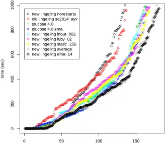
Note that a virtual best solver of all uniform versions static-r would only solve a total of 191 instances. For practical considerations, a more interesting version of a virtual best solver might be obtained as follows. For each different bucket, pick the versionstatic-rthat performs best on the specific bucket. This probably comes close to the performance a portfolio solver, consisting of all static-r, would achieve in practice. In our experiments, this kind of virtual best solver would have solved 180 instances. This further emphasizes the effectiveness of the dynamic restart strategy in finding optimal restart intervals. To give an overall impression, Figure5contains a cactus plot for a selected subset of the discussed solvers.
0 50 100 150
0
200
400
600
800
1000
solved SAT competition 2014 application instances (ordered by solving time)
time (sec)
●●●●●●●●●●●●●●●●●●●●●●●●●●●●●● ●●●●●●●●●●●●●
●●●●●● ●●●●●●
●●●●● ●●
●● ●●●
●●●●● ●●●●●
●●●●● ●●●●
●●● ●●●●●●
●●●● ●●
●●● ●●●
●●● ●●●●●●
● ●●
● ●
●●●●● ●●●
●● ●●●
●
● new lingeling norestarts
old lingeling sc2014−ayv glucose 4.0
glucose 4.0 ema new lingeling inout−002 new lingeling luby−02 new lingeling static−256 new lingeling average new lingeling ema−14
Figure 5: Cactus plot for a selected subset of solvers.
Lingeling. To be independent from a specific floating point representation, EMA calculation in Lingeling is based on fixed point operations. In our actual implementation of forcing restarts in ema-X, we compute two EMAs, a slow (low frequency) EMA s and fast (high frequency) EMAf, both over the actual glucose levelg(the LBD). The slow EMA will fluctuate less (with lower frequency), since it is smoothing more, while the fast EMA will fluctuate more (with higher frequency), since it is smoothing less. Recent glucose levels are less important for the slow version and more important for the fast one.
As already mentioned, we useαf = 2−5 for the short term EMAf, replacing the SMA for
forcing restarts. For Lingeling versionsema-X, we further rely on a slow EMAsfor representing the long term average, instead of using an overall average (i.e., a CMA). In particular, we choose
αs = 2−X, which corresponds to a window size of 2X+1−1. The EMA implementation for
The 64 bit fixed point calculation of the two EMA values for forcing restarts looks as follows:
Fi+1= 227gi+ (1−2−5)Fi Si+1= 232−Xgi+ (1−2−X)Si,
This is following Donald Knuth’s implementation of our agility based restart strategy using fix point arithmetic, e.g., withf = 2−32F ands= 2−32S:
fi+1= 2−5gi+ (1−2−5)fi si+1= 2−Xgi+ (1−2−X)si,
If we abstract from the actual values, we have
fi+1=αfgi+ (1−αf)fi si+1=αsgi+ (1−αs)si,
withαf = 2−5 and αs= 2−X being the fast exponential smoothing factor and the slow one,
respectively. The basic idea is now, after at least a certain number of conflicts has passed (we use 50, as in the Glucose 2.3 implementation [3, 2]), to restart if f >1.15·sor, equivalently, if F > 1.15·S. The same kind of implementation is used for blocking restarts, with the corresponding values of α0 = 2−12 and c0 = 1.4, but comparing a single EMA to the current number of assigned variables.
As discussed above, initialization is non-trivial for an EMA. W.l.o.g., let us again consider the case of forcing restarts. To smooth the bias that is introduced by initializing the EMA value with the first glucose levelg1, we use a larger value forαin the beginning and only gradually reduce it. In particular, for calculating the (i+ 1)th EMA, we use α(i):= 2−i, untilα(i)≤α. This removes part of the bias from the first glucose level and distributes it in a smoother way. This kind of initialization is used for all EMAs in our implementation.
5
Conclusion
In this paper, we provided an extensive empirical evaluation of different restart strategies in the context of modern CDCL solvers. We first looked at static restart schemes. Our results show that, for uniform restart policies, the optimal interval size not only depends on the satisfiability status of a given instance, but also on the specific problem class. In particular, our solver versionstatic-256was the best performing one, regarding intervals with fixed size.
Comparing those results with non-uniform restart schemes, it turned out that previously most successful strategies, such as Luby restarts, did not give an additional benefit in com-bination with the current state-of-the-art solver Lingeling on recent competition benchmarks. Our best non-uniform version,luby-02, solved exactly as many instances as the best uniform one. Interestingly, the equally well-known inner/outer scheme actually performed worse. This emphasizes the need for occasional re-evaluation of well-known techniques in consideration of the steady changes made in modern CDCL solvers due to the ongoing development.
In a second part, we revisited the Glucose restart scheme, being the currently most successful dynamic strategy. Since solvers that used Glucose restarts were able to solve a substantial number of instances in the SAT competition 2014 that Lingeling versionsc14ayvwas not able to solve, we implemented a similar strategy in our new version average. Our experimental results show, that this version of Lingeling significantly outperforms all versions with static restart schemes, as well as the SAT competition version of Glucose.
proposed to use exponential moving averages, because of several desirable properties. In par-ticular, exponential moving averages do not require the implementation of a queue and, more important, gradually smooth the influence of earlier values.
The concerete implementation of the proposed exponential moving average version of Glu-cose restarts into Lingeling uses fixed point representation, which we described in detail. We further presented a possible technique for smoother initialization. Our evaluation shows that the resulting Lingeling versions improve state-of-the-art. For future work, further improve-ments of the current implementation, e.g., more sophisticated intialization techniques might be of interest. We also experimented with related concepts from statistical analysis, such as DEMAs (double exponential moving averages) and the MACD (moving average convergence/-divergence) indicator but, so far, were not able to achieve further improvements by doing so. Continuing research into this direction could also be part of future work. Aside from this, exhaustive evaluations on a broader range of benchmarks will increase robustness of solvers and prevent overtuning. Similarly, considering larger timeouts will be of interest. Preliminary experiments using older competition instances and a timeout of 5000 seconds seem to confirm the previous results also in a more general setting.
References
[1] Gilles Audemard and Laurent Simon. Predicting learnt clauses quality in modern SAT solvers. In Craig Boutilier, editor,IJCAI 2009, Proceedings of the 21st International Joint Conference on Artificial Intelligence, Pasadena, California, USA, July 11-17, 2009, pages 399–404, 2009. [2] Gilles Audemard and Laurent Simon. Refining restarts strategies for SAT and UNSAT. In Michela
Milano, editor,Principles and Practice of Constraint Programming - 18th International Confer-ence, CP 2012, Qu´ebec City, QC, Canada, October 8-12, 2012. Proceedings, volume 7514 ofLecture Notes in Computer Science, pages 118–126. Springer, 2012.
[3] Gilles Audemard and Laurent Simon. Glucose 2.3 in the SAT 2013 Competition. In Balint et al. [4], pages 42–43.
[4] Adrian Balint, Anton Belov, Marijn J. H. Heule, and Matti J¨arvisalo, editors.Proceedings of SAT Competition 2013, volume B-2013-1 ofDepartment of Computer Science Series of Publications B. University of Helsinki, 2013.
[5] Anton Belov, Marijn J. H. Heule, and Matti J¨arvisalo, editors. Proceedings of SAT Competition 2014, volume B-2014-2 ofDepartment of Computer Science Series of Publications B. University of Helsinki, 2014.
[6] Armin Biere. Adaptive restart strategies for conflict driven SAT solvers. In Hans Kleine B¨uning and Xishun Zhao, editors,Theory and Applications of Satisfiability Testing - SAT 2008, 11th In-ternational Conference, SAT 2008, Guangzhou, China, 2008. Proceedings, volume 4996 ofLecture Notes in Computer Science, pages 28–33. Springer, 2008.
[7] Armin Biere. PicoSAT essentials. JSAT, 4(2-4):75–97, 2008.
[8] Armin Biere. Yet another local search solver and Lingeling and friends entering the SAT Compe-tition 2014. In Belov et al. [5], pages 39–40.
[9] Armin Biere and Andreas Fr¨ohlich. Evaluating CDCL variable scoring schemes. In Marijn Heule and Sean Weaver, editors, Theory and Applications of Satisfiability Testing - SAT 2015 - 18th International Conference, Austin, TX, USA, September 24-27, 2015, Proceedings, volume 9340 of Lecture Notes in Computer Science, pages 405–422. Springer, 2015.
[10] Armin Biere, Marijn J. H. Heule, Matti J¨arvisalo, and Norbert Manthey. Equivalence checking of HWMCC 2012 circuits. In Balint et al. [4], page 104.
[12] Niklas E´en and Niklas S¨orensson. An extensible SAT-solver. In Enrico Giunchiglia and Armando Tacchella, editors,Theory and Applications of Satisfiability Testing, 6th International Conference, SAT 2003. Santa Margherita Ligure, Italy, May 5-8, 2003 Selected Revised Papers, volume 2919 ofLecture Notes in Computer Science, pages 502–518. Springer, 2004.
[13] Daniel Frost, Irina Rish, and Llu´ıs Vila. Summarizing CSP hardness with continuous probability distributions. In Benjamin Kuipers and Bonnie L. Webber, editors,Proceedings of the Fourteenth National Conference on Artificial Intelligence and Ninth Innovative Applications of Artificial In-telligence Conference, AAAI 97, IAAI 97, July 27-31, 1997, Providence, Rhode Island., pages 327–333. AAAI Press / The MIT Press, 1997.
[14] Carla P. Gomes, Bart Selman, Nuno Crato, and Henry A. Kautz. Heavy-tailed phenomena in satisfiability and constraint satisfaction problems. J. Autom. Reasoning, 24(1/2):67–100, 2000. [15] Jinbo Huang. The effect of restarts on the efficiency of clause learning. In Manuela M. Veloso,
edi-tor,IJCAI 2007, Proceedings of the 20th International Joint Conference on Artificial Intelligence, Hyderabad, India, January 6-12, 2007, pages 2318–2323, 2007.
[16] Matti J¨arvisalo, Marijn J. H. Heule, and Armin Biere. Inprocessing rules. In Bernhard Gramlich, Dale Miller, and Uli Sattler, editors,Automated Reasoning - 6th International Joint Conference, IJCAR 2012, Manchester, UK, June 26-29, 2012. Proceedings, volume 7364 of Lecture Notes in Computer Science, pages 355–370. Springer, 2012.
[17] Robert G. Jeroslow and Jinchang Wang. Solving propositional satisfiability problems. Annals of Mathematics and Artificial Intelligence, 1(1-4):167–187, 1990.
[18] Henry A. Kautz, Eric Horvitz, Yongshao Ruan, Carla P. Gomes, and Bart Selman. Dynamic restart policies. In Rina Dechter and Richard S. Sutton, editors,Proceedings of the Eighteenth National Conference on Artificial Intelligence and Fourteenth Conference on Innovative Applications of Artificial Intelligence, July 28 - August 1, 2002, Edmonton, Alberta, Canada., pages 674–681. AAAI Press / The MIT Press, 2002.
[19] Donald E. Knuth. The Art of Computer Programming, Volume II: Seminumerical Algorithms, 2nd Edition. Addison-Wesley, 1981.
[20] Jia Hui Liang, Vijay Ganesh, Ed Zulkoski, Atulan Zaman, and Krzysztof Czarnecki. Understand-ing VSIDS branchUnderstand-ing heuristics in conflict-driven clause-learnUnderstand-ing SAT solvers. In Nir Piterman, editor, Hardware and Software: Verification and Testing - 11th International Haifa Verification Conference, HVC 2015, Haifa, Israel, November 17-19, 2015, Proceedings, volume 9434 ofLecture Notes in Computer Science, pages 225–241. Springer, 2015.
[21] Michael Luby, Alistair Sinclair, and David Zuckerman. Optimal speedup of las vegas algorithms. InISTCS, pages 128–133, 1993.
[22] Jo˜ao P. Marques-Silva, Inˆes Lynce, and Sharad Malik. Conflict-driven clause learning SAT solvers. In Armin Biere, Marijn J. H. Heule, Hans van Maaren, and Toby Walsh, editors,Handbook of Satisfiability, volume 185 of Frontiers in Artificial Intelligence and Applications, pages 131–153. IOS Press, 2009.
[23] Jo˜ao P. Marques-Silva and Karem A. Sakallah. GRASP: A search algorithm for propositional satisfiability. IEEE Trans. Computers, 48(5):506–521, 1999.
[24] Matthew W. Moskewicz, Conor F. Madigan, Ying Zhao, Lintao Zhang, and Sharad Malik. Chaff: Engineering an efficient SAT solver. In Proceedings of the 38th Design Automation Conference, DAC 2001, Las Vegas, NV, USA, June 18-22, 2001, pages 530–535. ACM, 2001.
[25] Chanseok Oh. MiniSat HACK 999ED, MiniSat HACK 1430ED and SWDiA5BY. In Belov et al. [5], pages 46–47.
editors,Theory and Applications of Satisfiability Testing - SAT 2008, 11th International Confer-ence, SAT 2008, Guangzhou, China, May 12-15, 2008. Proceedings, volume 4996 ofLecture Notes in Computer Science, pages 271–276. Springer, 2008.
[28] Peter van der Tak, Antonio Ramos, and Marijn J. H. Heule. Reusing the assignment trail in CDCL solvers. JSAT, 7(4):133–138, 2011.