Research Journal
Volume 11, Issue 2, June 2017, pages 51–57
DOI: 10.12913/22998624/68730 Research Article
APPLICATION OF AN EQUIVALENT TRUSS MODEL FOR DETERMINING
THE STRESS STATE IN MULTI-PHASE MATERIALS WITH CELLULAR
AUTOMATA METHOD
Anna Staszczyk1, Jacek Sawicki1
1 Institute of Materials Science and Engineering, Faculty of Mechanical Engineering, Lodz University of
Technology, 1/15 Stefanowskiego Street, 90-924 Łódź, Poland, e-mail: [email protected]
ABSTRACT
The Cellular Automata represent a universal method of modelling and simulation. They enable the performance of calculations for even the most complex processes and phenomena. They are also used successfully in mechanical and material engineering. In this paper, the concept of application of the Cellular Automata method for simulat-ing the behaviour of material under stress is presented. The proposed numerical algo-rithm created performs a number of calculations of local stress states in the structure of precipitation hardened material. The principle of its operation is based on the ap-plication of the equivalent truss model, which is often used in the optimisation and de-sign of structures. In this paper, this model was used to simulate a system embodying a
section of the material containing various phases with different mechanical properties.
Keywords: Cellular Automata, numerical methods, stress state, strength of materials, precipitation hardening.
INTRODUCTION
The equivalent truss model was applied suc-cessfully to optimise the structural topology. Op-timisation methods were applied to elements in both macro- and microscopic scale [1]. All the theoretical aspects of modern structural optimi-zation issues were described by Rozvany in his work [2]. In that work, this method is used to solve the stress state in a deformed material. The theoretical model is implemented into the algo-rithm based on the Cellular Automata method.
The notion of Cellular Automata
(abbrevi-ated as CA) was formul(abbrevi-ated for the first time in
1940s by John von Neumann, a mathematician and computer scientist of Hungarian origin. A cellular automaton is a self-replicating system consisting of a cellular grid where every cell
has a finite number of states [3]. Such a grid can
have any number of dimensions. Automatons in one, two or three dimensions are those used the
most often. For every cell, the so-called neigh-bourhood is defined, that is, a set of cells that
remain in direct contact with it and the states of which are taken into account when establishing the state of the cell. A cellular automaton is a dis-crete model. Its space, number of possible states
and time during which it evolves are finite and
countable. The system evolution consists in the cell state being established in every pass on the basis of state of neighbourhood cells and state of the cell concerned during the previous step. The
above dependencies are defined via passage rules.
The principles of operation of cellular automata
have been widely documented [3, 4, 5].
The equivalent truss model is based on the assumption that a solid body, being a continuous centre, can be presented in the form of a truss
with a specified geometry [6]. Cellular Automa -ta are a frequently used method of implementing a model into numerical algorithms. Using them for the above mentioned purpose was descried Received: 2017.01.23
The numerical model assumed writing an al-gorithm that creates the two-dimensional geom-etry of a multi-phase material and then executes a simulation of the material deformation process and calculates stresses at every point of the Cel-lular Automaton grid.
Computational domain
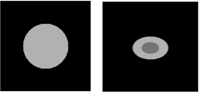
The computational domain of an automaton is constituted by a system which is a two-dimen-sional digital representation of a square section of the material containing a circular or elliptical hardening phase precipitate in its centre. The pre-cipitate geometry is created by the user who in-troduces its parameters into the software or estab-lished on the basis of a microscopic image of the actual particle observed. The types of geometry generated by the software include only circular or elliptical precipitates containing one or two phases of the material.
A cellular grid with a resolution of 200x200 is
imposed onto the geometry. Every cell has fixed
values of mechanical properties assigned,
de-pending on its affiliation to a given phase of the
material. A cell is embedded in the direct neigh-bourhood of the Moore type, i.e. it has 8 most ad-jacent neighbours.
The geometry is generated by the software in the form of a bitmap. Every single map pixel is a single automaton cell. The bitmap includes three colours, each of which corresponds to one of the material’s phases. Black represents the material’s
precipitates and sections of material. In reality, the scale of precipitate sizes in aluminium alloys is very small, which complicates the calculation of actual stresses.
Boundary conditions
A system which is the computational domain of an automaton is subjected to axial tensioning
with a fixed force until the moment of achieving
the deformation set. In the algorithm described, it was assumed that the lower edge of the system
remains immobile, fixed to the substrate. The de -formation is applied to the upper edge of the sys-tem. The value of this deformation is set by the user and expressed as a percentage. There are no boundary conditions on the side cells, so these are
not fixed and are free to move.
Calculations
To make this a problem suitable for Cellular
Automata calculation, we first have to change the
continuum body into an equivalent truss model. Every body cell is treated as a truss node con-nected to eight cells of the Moore neighbourhood
using rods with specific sections and material
constants. There exist forces in these truss mem-bers when these are elongated or shortened. This kind of model is easily implemented in a cellular automata scheme. We update every node by po-sitioning it so that the sum of the acting forces is zero. This also coincides with searching for the
point of minimal potential energy. After sufficient
iterations, the whole body will be very close to its point of minimal potential energy. This means we are converging on the actual solution. Of course this method needs a certain (large) amount of it-erations depending on the number of nodes.
As an illustration of this method, we
ana-lysed a simple structure. This structure is a flat
square made from a homogeneous material with Young’s modulus E1. In the middle, we model the precipitate by adding a ellipsoid area with a dif-ferent Young’s modulus E2. This is the most basic way we can model an alloy with a certain
cipitate on a microscopic scale. Of course, with
this method, any number of different configura -tions can be analysed, but this one can be easily checked analytically.
As we are modelling a continuum body as a truss model, we need to relate the thickness of this continuum body and the cross-sectional area of the truss members. These can then be used in the calculation of the stresses and forces in our truss model. We can model this as a superposi-tion of the diagonal and horizontal and vertical members. The members can be interpreted as the springs, with elastic constants corresponding with Young’s modulus of the phase material, con-necting the nodes being the cell centers [10]. The diagonal members have a cross-sectional area Ad and the horizontal and vertical members have a cross-sectional area Ao. These areas can be cal-culated by using the equivalence of strain energy between the truss cell and the continuum cell for given nodal displacements.
(1)
(2)
(3)
Where l and t are the height and the thickness of the cell.
The starting point of this method is the forc-es acting on a joint in the mforc-esh. Thforc-ese joints are equally spaced. We use each iteration of cellular automata to sequentially position the cell so that the sum of all forces is zero. This gives us a vec-tor equation and a closed expression for the new position of each cell. If we do enough iterations, the resulting positions of each of the joints will be without internal forces, so we will have found the solution to the problem.
Here we are using a Moore neighbourhood, so we have 8 forces coming from 8 members act-ing on each joint.
These are used in the force equations to deter-mine the stresses and thus the position where the force is zero. These equations can be rearranged in the x- and y-direction. From these we can di-rectly calculate the x- and y-position of each par-ticle in each iteration.
(4) where: E – Young’s modulus, A – member’s
cross-sectional area, ε – strain in a mem -ber, Fi – external force.
(5)
(6)
(7)
(8)
When the truss nodes change their location, the directional cosines for the constituent forces change their values. This results in the system balance location solution being reduced to a sys-tem of complex non-linear equations without an analytical solution. However, due to the fringe conditions adopted and the fact that the analy-sis is performed for a rigid continuous body, the angle values only change to a very minor extent. The changes in node location for a single algo-rithm iteration are at the level of 10-8. In view of
the above reasons it was assumed that omitting
the angle changes would not have any significant
impact on the simulation result. The system was
reduced to linear equations, where the θ angle is
always 45°. This type of solution is probably not going to perform well in the case of deformations of greater magnitude.
The original no-stress heights of the cells are equal to 1 (dimensionless). These can easily be adapted to the grid size. But as all formulas are
Fig. 2. Diagram of an equivalent truss model
sitions in the Cartesian coordinate system corre-spond with the coordinates of bitmap pixels (they
differ by one), this deformation can be calculated as the difference between two positions of neigh -bouring cells and their original, undeformed gap.
(9) The stress values are later calculated using Hooke’s law.
(10)
Convergence of the solution
In this method, each cell is dependent on the displacements of its neighbours to calculate its own displacement. For this we can use two
different calculation methods; both have their drawbacks as well as benefits. As we are using a
whole array of cells, we can calculate all of them in parallel or sequentially. Using parallel
comput-ing means we can use the true benefits of cellular
automata: the short calculation time, but this re-quires special code and implementation. We store the old array of cells and calculate the new array directly using the old one. This is called a Jacobi
iteration, but is inefficient for any process that
converges. If we only have a sequential processor,
we can help the rate of convergence by using the updated array of cells to calculate the new
posi-tions sequentially. This is called the Gauss-Seidel
iteration method. The new values are calculated
using the updated values. Smaller numbers of it -erations are required to obtain convergence. This however eliminates the possibility of using paral-lel computing [12].
The convergence criterion has been set at 10-6
* MAX (maximum value of the positional change in the last iteration in the system). For the method adopted, the convergence is achieved after about
130 000 iterations.
RESULTS
The calculations were performed assuming the mechanical properties for the 2024 aluminium alloy containing precipitates after ageing process-ing. The values of the Young module and
Pois-son coefficient for a given material are indicated
in Table 1. All the simulations were performed for the total deformation in a tensioning direction equal to 0.05%.
The simulation results are presented in the form of a bitmap imposed onto the geometry.
Fig. 5. Maps of σy stresses for a circular precipitate with diameter of 50px and an elliptical precipitate with the
same section area and aspect ratio of 3
Fig. 6. Profile of directional stresses going through the centre of a precipitate with diameter of 50 px
The calculation results for every automaton
cell are recorded in text files. By using the co -ordinates, it is possible to determine the stress
profile along the line going through the centre
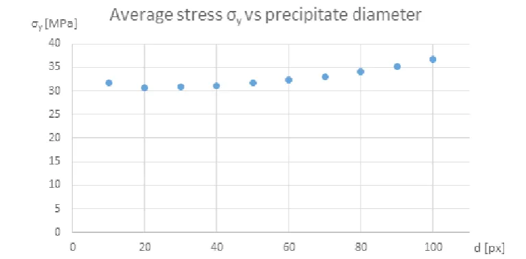
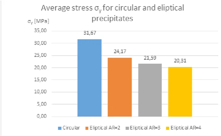
of precipitate. All the coordinates are measured in pixels. From the results obtained, the aver-age values of directional stresses inside the pre-cipitate were calculated. The results were com-pared among circular precipitates with various diameters in order to determine the relationship between the precipitate size and the stress gen-erated inside of it. Afterwards, the results were compared between a circular precipitate and el-liptical precipitates with the same section area
and different aspect ratios.
DISCUSSION AND CONCLUSIONS
A computational algorithm was calculated em-ploying the Cellular Automata method, being an iterative method of simulating the stresses in
two-phase materials. Simulations of axial tensioning of
material containing a single hard hardening phase precipitate on the example of the Al 2024 alloy were performed. In the case of the CA algorithm devel-oped it is possible to introduce our own geometries based on digital representations of microscopic im-ages of actual precipitates. The software is going to be developed within that scope in the future.
On the basis of the calculation results obtained the following conclusions were formulated:
• For identical values of total deformation the values of internal stresses of precipitates de-pend on their size. The larger the precipitate diameter, the higher the values of the direc-tional stresses.
• The distribution of stresses is influenced to a
great extent also by the shape of precipitates. For the precipitates with identical surface area, the stresses were inversely proportional to the ratio of precipitate width to its height.
REFERENCES
1. Kutylowski R.: Optymalizacja topologii
kontinu-um materialnego. Oficyna Wydawnicza Politech
-niki Wrocławskiej, 2004.
2. Rozvany G.: Aims, scope, methods, history and
uni-fied terminology of computer-aided topology optimi
-zation in structural mechanics. Structural and Multi -disciplinary Optimization, 21 (2), 2001, 90–108.
3. von Neumann J.: Theory of self-reproducing
au-tomata. Urbana: University of Illinois, 1969.
4. Wolfram S.: A New Kind of Science. Champaign:
Wolfram Media, 2002.
5. Dewei F.: Numerical computing method Based
on Cellular Automata. 3rd International Confer
-ence on Computer and Electrical Engineering. 53,
2012, 201–205.
6. Tatting B., Gurdal Z.: Cellular Automata for
De-sign of Two-dimensional Continuum Structures.
American Institute of Aeronautics and
Astronau-Fig. 8. Stress values for a circular precipitate and elliptical precipitates with differing aspect ratios and identical
tics, 8th Symposium on Multidisciplinary Analy -sis and Optimization, 2000.
7. Gurdal Z., Abdalla M.: Structural Design Using
Optimality Based Cellular Automata. American Institute of Aeronautics and Astronautics Paper,
1676, 2002.
8. Abdalla M. M., Gürdal Z.: Structural design using Cellular Automata for eigenvalue problems. Structural and Multidisciplinary Optimization, 25, 2003, 1–9.
9. Kita E., Toyoda T.: Structural design using cellular automata. Structural and Multidisciplinary Optimi -zation, 19 (1), 2000, 64–73.
10. Tatting B., Gurdal Z.: Cellular Automata for
De-sign of Truss Structures with Linear and Nonlinear
Response. American Institute of Aeronautics and Astronautics Paper, 2000.
11. Zakhama R., Abdalla M.: Topology design of geo-metrically nonlinear 2D elastic continua using CA
and an equivalent truss model. 11th AIAA/ISSMO
Multidiscipinary Analysis and Optimization
Con-ference, 2006, 1–10.