Evaluation of a multi-arm multi-stage Bayesian design for phase II drug selection trials – an example in hemato-oncology

R E S E A R C H A R T I C L E

Open Access

Evaluation of a multi-arm multi-stage

Bayesian design for phase II drug selection

trials

–

an example in hemato-oncology

Louis Jacob

, Maria Uvarova

, Sandrine Boulet

, Inva Begaj

and Sylvie Chevret

Abstract

Background:Multi-Arm Multi-Stage designs aim at comparing several new treatments to a common reference, in order to select or drop any treatment arm to move forward when such evidence already exists based on interim analyses. We redesigned a Bayesian adaptive design initially proposed for dose-finding, focusing our interest in the comparison of multiple experimental drugs to a control on a binary criterion measure.

Methods:We redesigned a phase II clinical trial that randomly allocates patients across three (one control and two experimental) treatment arms to assess dropping decision rules. We were interested in dropping any arm due to futility, either based on historical control rate (first rule) or comparison across arms (second rule), and in stopping experimental arm due to its ability to reach a sufficient response rate (third rule), using the difference of response probabilities in Bayes binomial trials between the treated and control as a measure of treatment benefit. Simulations were then conducted to investigate the decision operating characteristics under a variety of plausible scenarios, as a function of the decision thresholds.

Results:Our findings suggest that one experimental treatment was less efficient than the control and could have been dropped from the trial based on a sample of approximately 20 instead of 40 patients. In the simulation study, stopping decisions were reached sooner for the first rule than for the second rule, with close mean estimates of response rates and small bias. According to the decision threshold, the mean sample size to detect the required 0.15 absolute benefit ranged from 63 to 70 (rule 3) with false negative rates of less than 2 % (rule 1) up to 6 % (rule 2). In contrast, detecting a 0.15 inferiority in response rates required a sample size ranging on average from 23 to 35 (rules 1 and 2, respectively) with a false positive rate ranging from 3.6 to 0.6 % (rule 3).

Conclusion:Adaptive trial design is a good way to improve clinical trials. It allows removing ineffective drugs and reducing the trial sample size, while maintaining unbiased estimates. Decision thresholds can be set according to predefined fixed error decision rates.

Trial registration:ClinicalTrials.gov Identifier: NCT01342692.

Keywords:Bayesian, MAMS, Drop/select drug, Adaptive design

* Correspondence:[email protected] 1

Biostatistics and Clinical Epidemiology team (ECSTRA), of the Center of Research on Epidemiology and Biostatistics Sorbonne Paris Cité (CRESS; INSERM UMR 1153), Paris Diderot University, SBIM- Hôpital Saint Louis; 1, av Claude Vellefaux 75010, Paris, France

Full list of author information is available at the end of the article

Background

Adaptive designs for clinical trials that use features that change or “adapt” in response to information generated during the trial to be more efficient than standard ap-proaches [1] have been the focus of an abundant statis-tical literature since the 1970s. Among the wide range of adaptive designs, multi-arm multi-stage (MAMS) designs aim to compare several new treatments (multi-arm) to a common reference treatment to select or drop any treat-ment arm to move forward when evidence exists based on interim analyses (multi-stage). These designs have also been referred to as selection designs in phase II/III trials [2], randomized phase II screening trials [3] or select-drop designs [4]. Similarly to other adaptive designs, MAMS designs aim to decrease the time and number of patients required to move experimental treatments from develop-ment to a definitive assessdevelop-ment of benefit compared to the traditional approach, in which each drug is assessed through separate controlled trials. Improving the effi-ciency of clinical trials has been of prime interest in the development of anticancer therapies because multiple candidate anticancer agents are available for screening simultaneously due to the acceleration of drug devel-opment [3, 5]. However, although MAMS trials have gained popularity, they are still poorly used by practi-tioners. Notably, because of the number of arms and stages, MAMS trials appear more complex in design, conduct, and data analysis, with a broad variety of pro-posed versions [6–8]. All these proposed MAMS trials are faced with the issue of multiple testing due to com-parisons between active treatments and control treat-ment, or pairwise between all arms. Moreover, this multiplicity issue is increased by the repeated testing, resulting in stopping either the trial or merely the rele-vant arm, with a focus on sequential futility boundaries for lack of benefit adjusted so that the overall family-wise error rate is or is not controlled at a pre-specified αlevel.

We aimed at assessing how a Bayesian MAMS design may appear as an alternate way of handling such issues. Indeed, Bayesian designs are an efficient way to achieve valid and reliable evidence in clinical trials, given that the interpretation of the data is unrelated to preplanned stopping rules and is independent of the number of interim views [9, 10]. Such Bayesian approaches for MAMS trials have been rarely used, notably with one proposal for normal outcomes [11]. To allow a direct and simple use of the Bayes approach, we focused on the probability of success in binomial trials, restricting our considerations to conjugate beta priors. Moreover, it can then be easily updated along the trial, and allowance for early stopping for futility can be made. This setting of Bayes binomial trials was also recently used to com-pare the Bayesian approaches to frequentist hypothesis

testing in two-arm clinical trials [12]. Actually, our ap-proach could be also viewed as an extension to the MAMS trials with binary outcomes of that proposed by Zalavsky for two-arm trials [12]. Indeed, both ap-proaches use similar beta-binomial modeling (with in-tegers [12] or not as beta parameters), and posterior difference of beta as the quantity of interest for deci-sion making. However, while Zalavsky [12] focused on deriving one-sided superiority and non-inferiority Bayesian tests and their closeness to frequentist approaches, we pro-vided stopping rules as decision-tools for interim analyses due to the MAMS design, as Xie et al. did [13]. The scope for extending this approach to the comparison of different arms of experimental treatments against one control was considered below.

This paper was motivated by a phase II randomized controlled trial to compare on a binary outcome meas-ure, two experimental drugs with conventional azaciti-dine treatment for myelodysplastic syndrome patients, in which the main objective was to drop the experimental inefficacious arm. The trial was designed using a modi-fied two-stage Simon’s design [14], allowing with small sample sizes of 40 patients per arm in the first stage to control the type I error accurately at the pre-specified level of 0.15 with a statistical power of 0.80. At the end of this first stage, no decision of dropping any arm was made. We wondered whether the use of a Bayes ap-proach may have modified the design, and subsequent analyses.

Thus, the objective of this paper was to redesign the Bayesian adaptive design originally proposed by Xie, Ji and Tremmel for seamless phase I/II trials [13], focusing on the comparison of multiple experimental drugs to a control drug on a binary criterion measure.

First, we applied our design to the real dataset from the ongoing phase II randomized trial conducted on 120 patients that motivated this work. Then, we assessed its performance using a simulation study. Some discussion and conclusions are finally provided.

Methods

Motivating example

hypothesized that the response rate in the control group would be 0.30 and that a response rate of at least 0.45 would indicate that a combination was sufficiently promising to be included in further studies.

Bayesian multi-Arm multi-stage design

Let X denote the treatment arm, where X = 0 is the con-trol arm, and X = 1,…, K denote K distinct new drugs to be tested. Suppose thatnpatients are randomly allocated to each of the (K + 1) arms. For simplicity, let us con-sider a balanced design, although any imbalanced fixed design could be considered.

Consider a binary outcome, Y, where Y = 1 denotes a response to treatment and Y = 0 denotes the absence of a response. The observed number of responses among the nk patients allocated to arm k is given by

yk¼

Pn

i¼1yi1i∈k, where 1i∈k denotes the indicator

func-tion (1i∈k¼1 if the ith patient has been allocated to

arm k, and 0 otherwise). Note that the selection does not need to involve a measure of efficacy [2], so that response could be defined according to a toxicity grading scale.

We used a Bayesian inference framework, whereπk ¼P

Y ¼1jX ¼k

ð Þ denotes the probability of response in the arm X = k (k = 0,…, K). Using a beta Be(ak, bk) prior for

πk, the posterior probability ofπkis still a beta distribution given by Be(ak +yk,bk+nkyk) due to the natural

con-jugate property of the beta family for binomial sampling. The main aims of MAMS trials are to, over a range of K new treatments, select those that prove sufficiently efficacious and avoid those drugs that are unexpectedly ineffective. Let yki denote the number of responses

observed at stage i among the nki patients randomly

allocated to arm X =k(k = 0,…, K).

Thus, several stopping decision criteria were proposed, derived from the proposals of Xie [13].

First, the inefficacy of each drug was assessed by com-parison to some historical minimal value of interest, which was originally called the “minimum required treatment response rate”(MRT) by Xie et al. [13]. Thus, the futility rule (denoted as Rule 2 in [13]) is defined by the following posterior probability:

P πk<p0jyki;nki

>γ1 ð1Þ

where p0 denotes the MRT usually defined from some

historical control rates, and γ₁ is some threshold of a “high”probability of inefficacy.

In randomized phase II settings, the selection of a new drug is based on evaluating the potential benefits of the experimental treatment over the control arm [15]. Thus, one may consider dropping a new drug from further studies only if there is a rather low posterior probability that this drug is beneficial over the control by some

targeted minimal level while on the opposite selecting the drug if there is sufficient information to declare that one treatment is better than the other, that is when its benefit reaches a so-called“sufficient treatment response rate”(STR). Two resulting decision criteria and stopping rules were defined from the posterior distribution of the difference in response rates of the experimental over the control arm at the ith stage as follows:

P πk−π0>

△

<γ2 ð2Þ

P πk−π0>δjy_ki;nki

>γ3 ð3Þ

In the original paper [13], Eq. (2) is referred to as Rule 3, withΔset at the“targeted difference in response rate”, and Eq. (3) is referred to as Rule 4, with δ set at the STR. However, whereas Xie [13] used the Eq. (2) to define expansion for the seamless phase I/II design, in the present study, we only considered select/drop decisions due to the phase II design. More specifically, Eq. (2) attempts to assess the futility of experiencing experi-mental arm k given the posterior probability that its response rate compared to that observed in the con-trol arm is below some decision threshold; such a rule (2) can be considered as the posterior probability of the alternative hypothesis, as commonly used to evaluate the success of an experiment. Thus, such a rule was proposed to provide an answer closest to the frequentist setting where one wishes to test the null against the alternative. Note that when Δ= 0, the equation (2) reduces to the posterior probability that the experimental treatment is better than the control, a quantity that was first proposed in the setting of phase 2 single arm clinical trials [15] and more re-cently used to provide adaptive randomized allocation probability [16, 17]. By contrast, Eq. (3) aims at quan-tifying the posterior probability that response rate in experimental arm k is above that of the control arm by some sufficient treatment response rate. From a practical perspective, the alternative hypothesis in terms of differ-ences in response rates that aim for better performance (or non-inferiority) could be considered, and appear very natural in the clinical environment.

Contrary to the posterior density given in (1), the second and third rules involve the difference of two beta distributions (πk and π0, respectively), which is no

possible in a few special cases [20], while numerical integration is usually performed, like in [12, 15]:

Pðπk<π0þd y _k;nk;y0;n0

¼

Zp−d

0

F πkþdjakþyk; bkþnk−yk

f

ð

pja

þ

y

;

b

þ

n

−

y

Þ

ð4Þ

where F(|a,b) and f(|a,b) are the cumulative distribution function and the density of the beta random variable π~ Be(a,b), respectively.

The priors

Regarding the prior on the response probability, πk;

k¼0;…;K, the amount of past information is likely different according to the randomization arm. While it is expected that the elicitation of the prior on π0

could be based on previous trial results and expert opinion, that onπk;k>0, is likely to be less informative.

First, the use of flat non-informative priors was moti-vated by several considerations. It allows the posterior to be dominated by the data rather than by any prior over-optimistic views regarding the experimental arms. Thus, it insures that critical amount of clinical information is required as a basis for deciding whether the experimen-tal arm will be administered to a large number of patients in a Phase III clinical trial. Moreover, such domination by the data allows the trial results to be used by others who have their own priors [15].

However, it is widely recommended to use different prior densities to assess the robustness of the trial results. Thus, we performed sensitivity analyses to the

prior choice, using distinct beta distributions reflecting increased amount of prior information throughout the effective sample size (ESS) [21]. Given the ESS of a beta Be(a,b) prior is given by ESS=a+b, one may modifying the beta parameters for modifying the prior variance while the prior mean is fixed, providing sensitivity analyses to the prior information translated into a sam-ple size (Fig. 1). Prior mean was either “enthusiastic” or “skeptical”, as we did previously [22]. These terms “enthusiastic” and “skeptical” priors refer to either the optimistic view of a beneficial treatment effect at least equal to that expected when planning the trial, or to the pessimistic view of no treatment effect as compared to the control [23]. Both priors allow encompassing the hetero-geneity in physician prior opinion before to the trial.

Decision thresholds

To be applied, some arbitrary constants (further denoted as “design parameters”) must be defined. First, the choice of the minimal response rate (p0) could be guided by some historical controls or the clinical experience of the control group in the disease under study, and the response rate under the null hypothesis is commonly chosen in uncontrolled Phase II trials. Second, we choose Δ¼0 as a targeted minimal response rate; this value represents no difference between the treatments. δ_{¼0:15 was chosen as a sufficient response rate; this}

value would reflect a clinically important treatment effect. Both values delineate the underlying null and alternative hypotheses in a frequentist framework.

Otherwise, the number of design stages, that is, the frequency of the computation of the rules described above that conduct stopping decisions, should be defined. Moreover, the threshold values γ₁;γ₂ and γ₃

0 2 4 6 8 10

0

2

468

1

0

a

b

ESS=1 ESS=2 ESS=5 ESS=10

0.0 0.2 0.4 0.6 0.8 1.0

0.00

0.05

0.10

0.15

mean

variance

ESS=1 ESS=2 ESS=5 ESS=10

are statistical quantities that should be set to some pre-determined values allowing for the good performance of the design, likely related to the quantity of information in the trial (thus, of the entire sample size). Xie in 2012 [13] suggested thatγ₁ and γ₃ should be high (>0.8), and γ2 should be at most 0.10. Obviously, such values widely

govern the occurrence of false positive (or negative) decisions. Nevertheless, larger than traditional values of false positive rates are commonly used in MAMS settings, up to 0.50 at the first stage [8], notably because one wishes to make decision on dropping arms early while maintaining a low false negative decision rate.

Thus, we first proposed to compute the decision rules after every observed response in the trial and then attempt to define some criteria for design choices, and their impact in terms of sample size.

Results

Illustrative case study

We first apply the proposed design to the phase II randomized trial with K=2 new drugs compared against the control. The Jung trial design [14] was based on

p0=0.30 and δ=0.15, with type I and type II errors fixed at 0.15 and 0.20, respectively. Of the 120 enrolled pa-tients, 44 (36.7 %) exhibited a response, including 15 in arm A, 13 in arm B, and 16 in arm C, resulting in ob-served response rates of 0.3750, 0.3250 and 0.40, respectively.

Bayes analyses were applied, first using in each arm non-informative beta priors either the Jeffreys prior Be(1/2,1/2) or the uniform prior Be(1,1) resulting in ESS=1 or 2, respectively. Then, as reported above, a sensitivity analysis to the prior choice was performed; for the control arm, only skeptical priors - centered on the null (prior mean=0.3) hypothesis- were used, while both skeptical and enthusiastic – centered on the alter-native (prior mean=0.45) hypothesis- priors were de-fined. Prior effective sample size was set at 10 in control, and varied from 1 or 5 in experimental arms.

Figure 2 displays the prior and posterior distribution of response rates in each randomized arm at the end of enrollment, illustrating how the posterior distribution of each experimental arm was not markedly affected by the prior information as translated into the (prior) effective sample size or its location. At the end of the trial,

0.0 0.2 0.4 0.6 0.8 1.0

0123456

Non informative priors (Mean=0.5)

Probability of response ESS=1 ESS=2

0.0 0.2 0.4 0.6 0.8 1.0

0123456

Skeptical priors (Mean=0.3)

Probability of response ESS=10 (control) ESS=1 (experimental) ESS=5 (experimental)

0.0 0.2 0.4 0.6 0.8 1.0

0123456

Enthusiastic priors (Mean=0.45)

Probability of response ESS=10 (control) ESS=1 (experimental) ESS=5 (experimental)

0.0 0.2 0.4 0.6 0.8 1.0

0

1234

56

Posterior distributions

Probability of response ESS=1 (A) ESS=2 (A) ESS=1 (B) ESS=2 (B) ESS=1 (C) ESS=2 (C)

0.0 0.2 0.4 0.6 0.8 1.0

0

1

23456

Posterior distributions

Probability of response ESS=10 (A) ESS=1 (B) ESS=5 (B) ESS=1 (C) ESS=5 (C)

0.0 0.2 0.4 0.6 0.8 1.0

0

1

23456

Posterior distributions

Probability of response ESS=10 (A) ESS=1 (B) ESS=5 (B) ESS=1 (C) ESS=5 (C)

according to the prior, the posterior mean response rate ranged from 0.3600 to 0.3810 in arm A, from 0.3222 to 0.3389 in arm B, and from 0.3889 to 0.4056 in arm C (Table 1).

We retrospectively applied the decision rules defined in (1)-(3) with threshold values set at 0.9, 0.1 and 0.9, respectively. Figure 3 displays the evolution of the pos-terior probabilities and stopping criteria over time, when using non-informative priors.

The application of the first stopping criterion does not allow either arm to be eliminated, indicating that there is a small probability that either response rate is below the historical response rate of 0.30; indeed, the posterior esti-mates were close to and mainly above 0.30, except for arm B, where the response rate was lower than those of the other two arms for the 20 first enrolled patients (Fig. 2, left). This finding was illustrated in the second criterion computed over the trial, where the cut-off threshold of the

Table 1MDS results–Sensitivity analyses

Prior ESS Posterior mean Decision criteria

Arm A B C A B C A B C B C B C

Rule 1 Rule 1 Rule 1 Rule 2 Rule 2 Rule 3 Rule 3

MLE 0 0 0 0.3750 0.3250 0.4000

Non informative 1 1 1 0.3780 0.3293 0.4024 0.1505 0.3576 0.0863 0.3198 0.5906 0.0286 0.1197

2 2 2 0.3810 0.3333 0.4048 0.1384 0.3346 0.0789 0.3223 0.5894 0.0281 0.1161

Sk eptical 10 1 1 0.3600 0.3244 0.3976 0.1900 0.3833 0.0971 0.3575 0.6437 0.0310 0.1340

10 5 1 0.3600 0.3222 0.3976 0.1900 0.3885 0.0971 0.3465 0.6437 0.0262 0.1340

10 1 5 0.3600 0.3244 0.3889 0.1900 0.3833 0.1074 0.3575 0.6148 0.0310 0.1099

Enthusiastic 10 1 1 0.3600 0.3222 0.3889 0.1900 0.3885 0.1074 0.3465 0.6148 0.0262 0.1099

10 5 1 0.3600 0.3280 0.4012 0.1900 0.3640 0.0889 0.3716 0.6570 0.0338 0.1422

10 1 5 0.3600 0.3389 0.4012 0.1900 0.2996 0.0889 0.4128 0.6570 0.0393 0.1422

The first line refers to the maximum likelihood estimate of response probability of each treatment arm, while the other lines refer to Bayes posterior estimates with computed decision criteria based on different combinations of the priors

MLEmaximum likelihood estimate,ESSeffective sample size, Decision criteria use p0=0.3,Δ=0,δ*=0.15: p0refers to the minimum required treatment response rate of the first rule (Eq.1);Δto the targeted difference of the second rule (Eq.2), andδ* to the sufficient treatment response rate of the third rule (Eq.3)

0 10 20 30 40

0.0

0.2

0.4

0.6

0.8

1.0

Index

pA/pB/pC

A

B

C Posterior Response Rates

0 10 20 30 40

0.0

0.2

0.4

0.6

0.8

1.0

Index

Pr(Response)<p0

A

B

C Rule 1

0 10 20 30 40

0.0

0.2

0.4

0.6

0.8

1.0

Observations

Pr(Difference>0)

B vs A

C vs A Rule 2

0 10 20 30 40

0.0

0.2

0.4

0.6

0.8

1.0

Observations

Pr(Difference>STR)

B vs A

C vs A Rule 3

second decision criterion was crossed for arm B after 5, 13, 14, 18, and 22 enrolled patients in that arm, illustrating a low (<0.10) posterior probability that the response rate in that arm was above that observed in the control. As ex-pected, the third decision criterion never required that the study be stopped with the conclusion that the benefit of any experimental arm was at least the 0.15 expected. Note that all the three decision criteria at the end of the trial were slightly affected by the prior, with close values that do not modify any decision (Table 1).

These findings suggest that arm B could have been dropped from the trial based on a sample of approxi-mately 20 instead of the 40 actually recruited patients, although further results (with a sample size of at least 25 patients) do not confirm such a decision. This could be related to some “drift” towards improved response rates over the course of the trial. This may also point out that the probability in Eq. (2) can be highly variable in the beginning of the trial when the number of patients is small, resulting in possibly false decisions [17].

We thus decided to assess the performances of this approach and more specifically to assess the quantity of information required to drop an ineffective arm or an

efficacious arm, according to decision thresholds related to false decision probabilities.

Simulation study

Simulation settings

Once the Bayesian design has been structured, statisticians use simulations and adjust tuning parameters to comply with a set of targeted operating characteristics. Thus, we assessed the operating characteristics of the proposed MAMS design through simulations that mimic the MSD trial, although with clear-cut ineffective or effective drugs, and in which stopping decision criteria (1)-(3) were applied. We considered several situations of drug inefficacy, that is, when the benefit in terms of response rate was null or below that expected of 0.15 (true benefit set at 0, 0.05, and 0.10 compared to an expected response rate of 0.30), and situations of drug efficacy (true benefit at 0.15, 0.20, 0.25, 0.30 and 0.45, over the 0.30 expected response rate). Moreover, among the K=2 new drugs, several scenarios combining these various treatment benefits were distinguished, either similar across new drugs or not. The first scenario simulated the case in which the efficacies of treatments B and C were similar

Table 2Simulation results in terms of absolute bias based on a fixed sample size for increasing benefit of the experimental arm–all priors on pk(k=A,B,C) are non-informative Be (1,1) priors; p0=0.30;n=40 or 100 patients per arm

Sample size True benefit Posterior mean estimate biases Mean square errors Decision criterion 1 Criterion 2 Criterion 3

dB pA pB pA pB A B B B

40 0.00 0.0086 0.0090 0.0048 0.0048 0.4850 0.4835 0.5012 0.1414

0.05 0.0082 0.0078 0.0048 0.0052 0.4854 0.2982 0.6358 0.2399

0.10 0.0100 0.0042 0.0050 0.0054 0.4798 0.1632 0.7440 0.3518

0.15 0.0097 0.0014 0.0049 0.0055 0.4798 0.0753 0.8352 0.4803

0.20 0.0098 −0.0001 0.0049 0.0057 0.4795 0.0297 0.9028 0.6132

0.25 0.0096 −0.0013 0.0049 0.0056 0.4800 0.0093 0.9477 0.7322

0.30 0.0095 −0.0049 0.0049 0.0055 0.4804 0.0027 0.9731 0.8271

0.35 0.0088 −0.0070 0.0048 0.0051 0.4841 0.0005 0.9886 0.8999

0.40 0.0109 −0.0087 0.0048 0.0047 0.4749 0.0001 0.9958 0.9477

0.45 0.0092 −0.0116 0.0049 0.0043 0.4808 0.0000 0.9984 0.9755

100 0.00 0.0042 0.0032 0.0020 0.0020 0.4863 0.4925 0.4960 0.0460

0.05 0.0037 0.0030 0.0020 0.0022 0.4885 0.2156 0.7042 0.1363

0.10 0.0040 0.0014 0.0020 0.0023 0.4866 0.0661 0.8503 0.2896

0.15 0.0038 0.0012 0.0020 0.0024 0.4881 0.0128 0.9404 0.4925

0.20 0.0040 −0.0003 0.0020 0.0024 0.4858 0.0015 0.9807 0.6875

0.25 0.0027 −0.0009 0.0020 0.0023 0.4947 0.0001 0.9950 0.8473

0.30 0.0046 −0.0017 0.0020 0.0023 0.4836 0.0000 0.9989 0.9362

0.35 0.0042 −0.0032 0.0020 0.0022 0.4856 0.0000 0.9998 0.9792

0.40 0.0032 −0.0037 0.0020 0.0021 0.4922 0.0000 1.0000 0.9952

0.45 0.0036 −0.0047 0.0020 0.0018 0.4897 0.0000 1.0000 0.9992

to that of treatment A (πB¼πC ¼πA ). In further

scenarios, we simulated the case in which only arm B was more efficient than A (πC¼πA;πB¼πAþdB). In

the latter, we simulated the cases where both B and C treatments had a higher probability of response than A (πC ¼πAþdC;πB¼πAþdB).

We simulated samples ofnpatients. In each simulation, the treatment arm was generated from a multinomial distribution mult(n;13;

1 3;

1

3), and the response-indicating

efficacies were generated from Bernoulli distributions B(πk).

For each scenario, data were analyzed using Bayesian inference. The priors of πk were non-informative beta

Be(1,1). Posterior probabilities in (1) were easily obtained as beta cumulative density functions, whereas those of (2) and (3) required numerical integration–see Eq. (4). We first computed those criteria for fixed sam-ple sizes. Then, any arm could be dropped if evidence suggested that it was unlikely to be effective (futility rules 1 and 2) or if sufficient evidence of effectiveness over the control had already been determined (rule 3). Furthermore, to take into account the high variability in

differences of beta distributions based on small samples [16], those rules only applied once at least 15 patients had been enrolled in each arm.

A total of N=10,000 independent replications were performed, with the results averaged across the N re-peated simulations. In all simulations, design parame-ters were set to be constant at p0=0.30, △¼0 and δ_{¼0:15 unless otherwise specified.}

All analyses were performed using the R statistical software (http://www.R-project.org/).

Simulation results

Threshold calibration

To determine the decision thresholds, as suggested by Xie [13], some simulations were first performed, con-sidering a 2 fixed parallel arm designs based on n=40 and n=100 patients per arm (Table 2). In all cases, biases were low, mainly below 0.01 (when n=40) or 0.005 (when n=100), with lower mean square errors (MSEs). The first decision criterion, that is, the posterior probability that the response rate was lower than 0.3 was nearly equal to 0.5 in the control arm or when there was

0 20 40 60 80 100

0.0

0.2

0.4

0.6

0.8

1.0

Sample size

Deci

si

on cri

teri

on

1

dB=-0.20 dB=-0.15 dB=-0.10 dB=-0.05 dB=0.00

0 20 40 60 80 100

0.0

0.2

0.4

0.6

0.8

1.0

Sample size

Deci

si

on cr

it

er

ion

2

dB=-0.20 dB=-0.15 dB=-0.10 dB=-0.05 dB=0.00

0 20 40 60 80 100

0.0

0.2

0.4

0.6

0.8

1.0

Sample size

Deci

si

on cr

it

er

ion

3

dB=0.45 dB=0.40 dB=0.35 dB=0.30 dB=0.25 dB=0.2 dB=0.15

no drug benefit (dB=0), as expected, and then decreased from 0.30 (when dB=0.05 andn=40) down to 0.01 (when dB=0.25) to reach 0 when dB=0.45. In parallel, the difference between the probabilities of a response for B over the control arm A increased with the benefit of B. Moreover, a larger sample size led to a higher probability of detecting a smaller benefit, so that for a given bene-fit, the decision threshold depends on the amount of information.

We thus computed the three decision criteria according to the true benefit of the experimental arm (dB ranging from −0.2 to 0.45) and to the sample size (ranging from 10 to 100 patients per arm), each based on 10,000 inde-pendent replications (Fig. 4). Left plots of Fig. 4 quantify to what extent the stopping rule (1) is influenced by the sample size and the actual benefit of the experimental treatment arm – beside the threshold cut-off value, ex-pectedly. Notably, it shows that a threshold of 0.95 with samples ofn=40 patients per arm, allows on average arms with response rates below 0.15 of that expected to be dropped, while those with response rates below 0.10 could be dropped only when the sample size reached

n=100. Similarly, when the experimental arm is com-pared to the control (middle plots), rule 2 evaluating the futility of trial continuation, with a 0.05 threshold,

allows on average arms with a response probability at least 0.20 below that of control to be dropped when the sample size was n=40, and those with response probability 0.15 below to the control when n=100. In contrast, a threshold of 0.95 for rule 3 (right plots) will enable one to determine that the benefit of the experimental over the control is at least 0.40 with

n=40, and nearly 0.30 with n=100.

Obviously, when the threshold values were less stringent, the increased ability of the design in dropping less different arms compared to the control could be counterbalanced by its increase propensity of dropping efficacious arms. This was the further aim of the simu-lation study to assess those false (positive or negative) decision rates.

Assessing false decision rates

Tables 3, 4 and 5 summarize the simulation results for the arms dropped at the end of the first stage and the absolute bias in their treatment effect estimates on the definitive outcome at the stopping decision based on rules 1, 2 and 3, respectively, when the sample size was set atn=40, 100 per arm, and the threshold values were set at stringent values, that is, of γ₁¼0:95, γ₂¼0:05 andγ₃¼0:95:

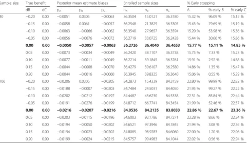
Table 3Simulation results for dropping treatment arms based on the first rule (R1) and the absolute bias for such arms in the estimated treatment effect at the time of dropping decision–all priors on pk(k=A,B,C) are non-informative beta(1, 1) priors, when decision threshold is set at 0.95

Sample size True benefit Posterior mean estimate biases Enrolled sample sizes % Early stopping

dB dC pA pB pC nA nB nC A % early B % early C

40 −0.20 0.00 −0.0051 0.0305 −0.0063 36.3504 15.0121 36.3180 15.32 % 96.09 % 15.15 %

−0.15 0.00 −0.0058 0.0061 −0.0057 36.2548 21.3829 36.3305 15.43 % 79.69 % 15.19 %

−0.10 0.00 −0.0063 −0.0066 −0.0062 36.3540 27.9657 36.3594 15.20 % 53.98 % 15.36 %

−0.05 0.00 −0.0056 −0.0076 −0.0072 36.2719 33.0725 36.2428 15.44 % 30.66 % 15.86 %

0.00 0.00 −0.0050 −0.0057 −0.0063 36.2726 36.4040 36.4653 15.77 % 15.11 % 14.85 %

0.05 0.00 −0.0073 −0.0034 −0.0049 36.2420 38.1107 36.3738 15.75 % 7.33 % 15.23 %

0.10 0.00 −0.0077 −0.0011 −0.0049 36.2214 39.1845 36.3761 15.91 % 2.92 % 14.88 %

0.15 0.00 −0.0044 −0.0008 −0.0070 36.4279 39.6107 36.2580 14.86 % 1.35 % 15.47 %

0.20 0.00 −0.0044 −0.0016 −0.0060 36.3945 39.8325 36.3640 15.06 % 0.55 % 15.29 %

100 −0.20 0.00 −0.0206 0.0305 −0.0205 84.2873 15.4339 84.3159 22.80 % 99.99 % 22.82 %

−0.15 0.00 −0.0188 −0.0007 −0.0203 84.7484 24.5031 84.4050 21.95 % 99.27 % 22.22 %

−0.10 0.00 −0.0202 −0.0212 −0.0197 84.4487 43.6230 84.5338 22.31 % 85.84 % 22.44 %

−0.05 0.00 −0.0191 −0.0276 −0.0199 84.8712 66.7741 84.3454 21.99 % 52.46 % 22.57 %

0.00 0.00 −0.0216 −0.0207 −0.0216 84.0536 84.2135 83.8033 22.86 % 22.67 % 23.36 %

0.05 0.00 −0.0203 −0.0115 −0.0196 84.6003 93.1786 84.7271 22.28 % 8.66 % 22.24 %

0.10 0.00 −0.0194 −0.0050 −0.0202 84.6521 97.3946 84.1845 21.94 % 3.08 % 22.76 %

0.15 0.00 −0.0194 −0.0023 −0.0202 84.8085 98.9283 84.6060 22.00 % 1.20 % 22.06 %

0.20 0.00 −0.0199 −0.0024 −0.0215 84.5757 99.4983 84.1044 22.02 % 0.56 % 22.94 %

As expected, when the treatment was less efficacious than expected, the first rule allowed the trial to be stopped early in 30.7–52.5 % of cases when the absolute difference in response rates was 5 %, to 96–99 % of cases when the absolute difference was down to 20 % (Table 3). The mean sample size required to detect inefficacy was 25 patients for a decrease of 0.15 in response rates, down to 15 for a 0.20 decrease. Otherwise, the false negative stopping rates due to this first rule in the case of beneficial treatment were low, with values of approxi-mately 15–23 % when there was no benefit, less than 10 % when the benefit was 5 %, and less than 1 % for higher benefits (Table 3).

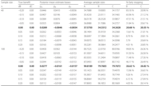
To handle the control arm, rule 2 was then applied to detect the lack of treatment benefit (Table 4). Com-pared to the previous first rule, a decision of stopping early in case of actual lower response rates in the ex-perimental group than in the control group appears to be reached similarly for small differences, with, for in-stance, a decision to stop in 32 % of cases compared to 31 % in the case of a 5 % response rate below that of the control forn=40 and in 46 % of cases compared to 52 % for n=100. In contrast, false negative decisions of dropping the arm were increased compared to rule 1 in

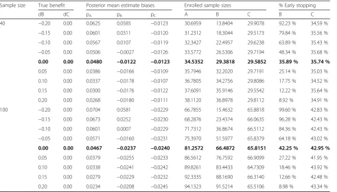
the same situation; for instance, for a minor benefit of 5 %, the second rule incorrectly proposes stopping for futility in 13–16 % of cases compared to 7–9 % based on the first rule when n=40 and n=100, respectively. Expectedly, when γ₂¼0:10, the results were modified, with lower false decision rates (Table 6).

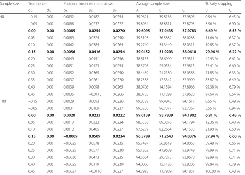
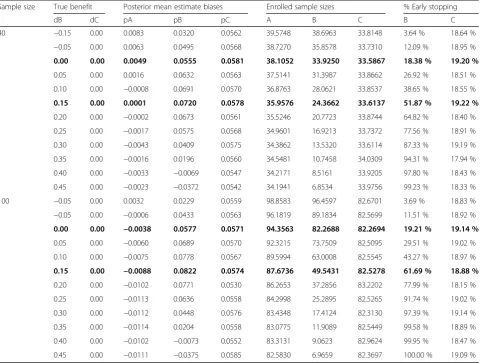
Finally, when evaluating the third rule in detecting true benefits, the average sample sizes were decreased to about 10 patients per arm when the absolute benefit increased to 45 %, while the false positive rate was only 6–7 % in the case of no benefit, likely related to the threshold probability of γ₃¼0:90 (Table 5). As expected, these figures were modified when using a less stringent probability threshold ofγ₃¼0:80 where the false positive rate reached 18–20 % in absence of any benefit (Table 7).

Discussion

There has been increasing evidence that the effectiveness of clinical trials can be improved by adopting a more in-tegrated model that increases flexibility and maximizes the use of accumulated knowledge. We focused this work on adaptive MAMS designs to select effective drugs among a fixed set of new drugs compared to a

Table 4Simulation results for dropping treatment arms based on the second rule (R2) and the absolute bias for such arms in the estimated treatment effect at the time of dropping decision–all priors on pk(k=A,B,C) are non-informative beta(1,1) priors, when decision threshold is set at 0.05

Sample size True benefit Posterior mean estimate biases Average sample sizes % Early stopping

n dB dC pA pB pC A B C B C

40 −0.20 0.00 0.0446 0.0410 −0.0036 34.7688 19.0005 34.1757 83.18 % 20.90 %

−0.15 0.00 0.0407 0.0196 −0.0049 35.4230 23.9111 34.1465 65.96 % 21.12 %

−0.10 0.00 0.0384 0.0076 −0.0045 36.0178 28.2528 33.9857 47.31 % 21.51 %

−0.05 0.00 0.0325 0.0004 −0.0039 36.8988 31.7086 34.2757 31.84 % 20.67 %

0.00 0.00 0.0289 −0.0046 −0.0034 37.5750 34.3312 34.2628 20.68 % 20.55 %

0.05 0.00 0.0262 −0.0053 −0.0046 38.1404 35.9159 34.2368 13.61 % 21.01 %

0.10 0.00 0.0212 −0.0068 −0.0038 38.6097 37.1804 34.2661 8.79 % 20.81 %

0.15 0.00 0.0184 −0.0079 −0.0043 39.0075 38.0515 34.3098 5.79 20.69 %

0.20 0.00 0.0163 −0.0098 −0.0051 39.2281 38.5864 34.2477 4.01 % 20.85 %

100 −0.20 0.00 0.0458 0.0362 −0.0144 80.7525 22.0750 80.0766 99.05 % 26.36 %

−0.15 0.00 0.0427 0.0103 −0.0153 81.9307 34.6011 79.9595 91.50 % 26.58 %

−0.10 0.00 0.0418 −0.0063 −0.0152 83.5055 51.2404 79.0897 71.48 % 27.30 %

−0.05 0.00 0.0344 −0.0142 −0.0153 87.6493 67.8997 80.1142 46.17 % 26.49 %

0.00 0.00 0.0277 −0.0161 −0.0157 90.8189 79.7603 79.7672 26.62 % 26.82 %

0.05 0.00 0.0247 −0.0149 −0.0154 93.1423 86.5031 79.4970 15.96 % 26.65 %

0.10 0.00 0.0202 −0.0130 −0.0157 95.3857 91.6455 78.7749 9.26 % 27.54 %

0.15 0.00 0.0154 −0.0119 −0.0155 96.8064 94.2754 79.4074 6.15 % 27.04 %

0.20 0.00 0.0112 −0.0100 −0.0147 97.8693 96.1853 80.1669 4.03 % 26.14 %

control. So-called screening or select/drop designs aim at proposing changes in treatment regimens with the possible elimination of a treatment group based on in-formation derived from accumulated data. Such designs appear particularly useful for rapidly evolving interven-tions and drugs, especially when outcomes occur suffi-ciently soon to permit adaptation of the trial design. This setting in which several treatments are compared to a single control allows heterogeneity in patient popu-lations and disease courses to be considered [24, 25]. However, the heterogeneity in objectives, design, data analysis, and reporting of these multi-arm randomized trials has recently been highlighted [26]. Moreover, in as-certaining which treatment modalities are most effective, the presence of K experimental arms also introduces complexity. We used a binary outcome measure, given that it appears to be the most widely used endpoint in phase II trials. Of note, such a binary criterion in MAMS has been used only in frequentist designs [6, 27].

Indeed, most of the proposed MAMS designs, including optimal designs, used a frequentist framework for inference

[4–8, 14, 28]. The application of Bayesian adaptive design methods has recently been advocated to maximize the knowledge-creating opportunity of a learning phase study [13]. Surprisingly, although several designs have used Bayes-ian adaptive allocation methods[17, 29], BayesBayes-ian adaptive designs in terms of sample size or treatment allocation have been proposed mainly in the early phases of cancer drug development, notably in the setting of seamless phase I/II trials [13]. In the MAMS setting, Bayesian adaptive phase II screening designs have been proposed only for selecting/ dropping arms using normal outcome measures [11], and more frequently by modifying the allocation probabilities to each arm. For instance, to select among treatment com-binations of multiple agents, patients were adaptively allo-cated to either one of the treatment combinations based on posterior probabilities of all hypotheses of superiority of each combination based on a continuous endpoint [29]. Even when comparing MAMS designs to adap-tive randomization designs, only the latter were based on Bayesian inference, whereas the former used test statistics from grouped sequential methods [27].

Table 5Simulation results evaluating Rule 3 when the threshold probability is set at 0.90

Sample size True benefit Posterior mean estimate biases Average sample sizes % Early stopping

dB dC pA pB pC A B C B C

40 −0.15 0.00 0.0092 0.0182 0.0254 39.9621 39.8136 37.9895 0.54 % 6.45 %

−0.05 0.00 0.0088 0.0237 0.0272 39.8054 38.8511 37.8795 3.56 % 6.90 %

0.00 0.00 0.0085 0.0254 0.0270 39.6095 37.9435 37.9783 6.69 % 6.53 %

0.05 0.00 0.0089 0.0324 0.0250 39.5103 36.5882 38.0288 11.66 % 6.37 %

0.10 0.00 0.0062 0.0384 0.0264 39.2740 34.3440 38.0311 19.85 % 6.37 %

0.15 0.00 0.0056 0.0416 0.0254 39.0452 31.9203 38.0610 29.96 % 6.22 %

0.20 0.00 0.0049 0.0451 0.0256 38.8153 28.6999 37.9511 42.93 % 6.61 %

0.25 0.00 0.0051 0.0423 0.0254 38.5798 25.0534 37.9815 57.41 % 6.60 %

0.30 0.00 0.0052 0.0369 0.0250 38.4489 21.2180 38.0583 71.85 % 6.33 %

0.35 0.00 0.0037 0.0261 0.0270 38.2338 17.3342 37.9999 83.87 % 6.49 %

0.40 0.00 0.0039 0.0098 0.0265 38.0706 14.1594 37.8966 92.38 % 6.79 %

0.45 0.00 0.0035 −0.0115 0.0266 38.0738 11.1299 37.9628 97.64 % 6.54 %

100 −0.15 0.00 0.0029 0.0093 0.0226 99.8389 99.4843 94.1617 0.55 % 6.49 %

−0.05 0.00 0.0031 0.0169 0.0237 99.3256 96.7377 93.7367 3.55 % 6.94 %

0.00 0.00 0.0020 0.0233 0.0222 99.0139 93.7839 94.1902 6.91 % 6.48 %

0.05 0.00 0.0013 0.0322 0.0224 98.3338 89.3276 94.1794 12.36 % 6.48 %

0.10 0.00 0.0012 0.0405 0.0227 97.6239 82.2664 94.1533 21.90 % 6.50 %

0.15 0.00 −0.0009 0.0509 0.0234 96.5788 71.2643 94.0376 37.94 % 6.60 %

0.20 0.00 −0.0025 0.0578 0.0235 95.7497 56.8519 94.0065 59.48 % 6.66 %

0.25 0.00 −0.0025 0.0577 0.0230 95.1262 41.9689 93.9749 79.99 % 6.71 %

0.30 0.00 −0.0030 0.0473 0.0235 94.5634 29.7273 93.9678 92.99 % 6.71 %

0.40 0.00 −0.0025 0.0119 0.0239 94.0066 15.1126 93.8206 99.84 % 6.79 %

0.45 0.00 −0.0027 −0.0110 0.0227 94.2995 11.7989 94.1851 100.00 % 6.48 %

We decided to focus on the select/drop decisions while preserving the equilibrium of sample allocation across arms. We first use stopping rules based on the posterior probability of inefficacy (or of over-toxicity), as previously performed in closed settings [30, 31]. Indeed, nearly all phase III trials include pre-specified inefficacy/futility interim monitoring rules to stop the trial early if the interim results strongly suggest that the experi-mental treatment has no benefit over the control [32]. In contrast, a phase II analysis in a phase II/III trial requires more evidence that the experimental treatment works better than the control [2]. Thus, we use the difference of response probabilities between the treated group and con-trol group as a simple Bayesian conditional measure of evidence regarding the treatment benefit. This method has been poorly used in a Bayesian context [12], possibly because the precise prior density of the difference of two independent beta is unknown. However, some analytical works have been published [18–20], and more recently, software to calculate the probability that one random vari-able is greater than another has been provided (http:// biostatistics.mdanderson.org/SoftwareDownload/). When this density can be approximated, it can be used in several important applications. This illustrates how Bayesian methods give direct answers to the questions that most people want to ask, such as“which treatment is the best” [10]. Moreover, the Bayesian tools enable decision making

based on the difference in response probabilities and the quantification of probabilities of benefit of each possible arm, which are more informative and transparent thanp -values. It could be combined with the adaptive design methodology to provide a very flexible and efficient deci-sion making process [33].

Due to the multiplicity of arms, we considered as the primary motivating design that of Xie et al. [13] who fo-cused on multiple dose levels, though our approach was close to that proposed by Zalavsky et al. for tow-arm tri-als [12]. Nevertheless, this exemplifies the large interests and clinical applications of such Bayesian designs, unfor-tunately still underused in clinical practice [34].

Since a common concern in Bayesian data analysis is that an inappropriately informative prior may unduly influence posterior inferences, we reran the analyses using different priors, possibly distinguishing various amounts of previous information across randomized arms as quantified by the effective sample size. This slightly modified the results of the clinical trial. We re-stricted our considerations to conjugate beta priors so that the prior probabilities of tested hypotheses could be transformed into Bernoulli trials with a theoretical (effective) sample size. This appeared an important issue when applying Bayesian methods in settings with a small to moderate sample sizes such as those pro-posed for MAMS [21].

Table 6Simulation results evaluating Rule 2 when the threshold probability is set at 0.10

Sample size True benefit Posterior mean estimate biases Enrolled sample sizes % Early stopping

dB dC pA pB pC A B C B C

40 −0.20 0.00 0.0625 0.0585 −0.0123 30.6959 13.8404 29.9078 92.23 % 34.59 %

−0.15 0.00 0.0601 0.0311 −0.0120 31.2312 18.3044 29.5173 79.84 % 35.56 %

−0.10 0.00 0.0567 0.0107 −0.0119 32.3427 22.4957 29.6238 63.89 % 35.43 %

−0.05 0.00 0.0506 −0.0027 −0.0126 33.5772 26.5306 29.7194 48.34 % 35.68 %

0.00 0.00 0.0480 −0.0122 −0.0123 34.5352 29.3818 29.5852 35.89 % 35.74 %

0.05 0.00 0.0386 −0.0166 −0.0109 35.7946 32.2020 29.7191 25.14 % 35.03 %

0.10 0.00 0.0337 −0.0178 −0.0107 36.7805 34.2756 29.8086 17.75 % 34.52 %

0.15 0.00 0.0300 −0.0176 −0.0122 37.6091 35.9146 29.5542 12.22 % 35.64 %

0.20 0.00 0.0268 −0.0180 −0.0111 38.1120 36.8978 29.8112 8.92 % 34.91 %

100 −0.20 0.00 0.0704 0.0581 −0.0229 66.7855 15.4632 65.8818 99.60 % 42.83 %

−0.15 0.00 0.0673 0.0252 −0.0230 68.2876 23.4374 66.0635 96.28 % 42.43 %

−0.10 0.00 0.0601 0.0007 −0.0229 71.7312 36.8674 66.5112 84.36 % 42.43 %

−0.05 0.00 0.0571 −0.0160 −0.0231 75.3970 51.5977 65.8379 64.18 % 43.02 %

0.00 0.00 0.0467 −0.0237 −0.0240 81.2572 66.4872 65.8151 42.25 % 42.95 %

0.05 0.00 0.0379 −0.0255 −0.0233 86.5612 76.7592 66.9099 27.22 % 41.95 %

0.10 0.00 0.0338 −0.0241 −0.0242 89.8261 83.4433 64.7309 18.46 % 43.92 %

0.15 0.00 0.0279 −0.0229 −0.0232 92.3335 88.1690 66.3140 12.66 % 42.48 %

0.20 0.00 0.0234 −0.0208 −0.0245 94.1323 91.5214 65.5106 8.98 % 43.34 %

Conclusions

Regardless of its inference, adaptive trial design is a methodologically sound way to improve clinical trials but adds significant complexity. This approach re-quires boundary parameters to be chosen for stopping decisions: Xie et al. in 2012 [13] reported the use of a high criterion for action (γ₂ =0.9) as a default value based on a maximum cohort size of 36 (with 24 treated with the active dose and 12 treated with pla-cebo), although calibration is often required. Thus, we calibrated the values of these thresholds according to the simulation study. Indeed, the choice of these thresholds is highly dependent on our desire to control false decision in either direction, as typically considered in early trial phases. Otherwise, combining stopping rules 1 and 2 appears to be another option to improve such a control [33].

Finally, this adaptive Bayesian approach in which existing information at the time of trial initiation is

combined with data accumulating during the trial has also been used to identify the treatments that are most beneficial for specific patient subgroups [35–38]. Such an approach, in the line of personalized medi-cine, appears to be an interesting research area to explore in the MAMS setting.

Abbreviations

B():Bernoulli distribution; Be(): beta distribution; ESS: effective sample size; MAMS: multi-arm multi-stage; MRT: minimum required treatment response; MSD: myelodysplastic syndrome; MSE: mean square error; mult(): multinomial distribution; STR: sufficient treatment response rate.

Acknowledgments

We wish to thank Professor Pierre Fenaux for providing access to this Phase II screening trial.

Funding

This work benefited from a grant from French Institute of Cancer, the INCA (2014–132, R14208KK).

Table 7Simulation results evaluating Rule 3 when the threshold probability is set at 0.80

Sample size True benefit Posterior mean estimate biases Enrolled sample sizes % Early stopping

dB dC pA pB pC A B C B C

40 −0.15 0.00 0.0083 0.0320 0.0562 39.5748 38.6963 33.8148 3.64 % 18.64 %

−0.05 0.00 0.0063 0.0495 0.0568 38.7270 35.8578 33.7310 12.09 % 18.95 %

0.00 0.00 0.0049 0.0555 0.0581 38.1052 33.9250 33.5867 18.38 % 19.20 %

0.05 0.00 0.0016 0.0632 0.0563 37.5141 31.3987 33.8662 26.92 % 18.51 %

0.10 0.00 −0.0008 0.0691 0.0570 36.8763 28.0621 33.8537 38.65 % 18.55 %

0.15 0.00 0.0001 0.0720 0.0578 35.9576 24.3662 33.6137 51.87 % 19.22 %

0.20 0.00 −0.0002 0.0673 0.0561 35.5246 20.7723 33.8744 64.82 % 18.40 %

0.25 0.00 −0.0017 0.0575 0.0568 34.9601 16.9213 33.7372 77.56 % 18.91 %

0.30 0.00 −0.0043 0.0409 0.0575 34.3862 13.5320 33.6114 87.33 % 19.19 %

0.35 0.00 −0.0016 0.0196 0.0560 34.5481 10.7458 34.0309 94.31 % 17.94 %

0.40 0.00 −0.0033 −0.0069 0.0547 34.2171 8.5161 33.9205 97.80 % 18.43 %

0.45 0.00 −0.0023 −0.0372 0.0542 34.1941 6.8534 33.9756 99.23 % 18.33 %

100 −0.05 0.00 0.0032 0.0229 0.0559 98.8583 96.4597 82.6701 3.69 % 18.83 %

−0.05 0.00 −0.0006 0.0433 0.0563 96.1819 89.1834 82.5699 11.51 % 18.92 %

0.00 0.00 −0.0038 0.0577 0.0571 94.3563 82.2688 82.2694 19.21 % 19.14 %

0.05 0.00 −0.0060 0.0689 0.0570 92.3215 73.7509 82.5095 29.51 % 19.02 %

0.10 0.00 −0.0075 0.0778 0.0567 89.5994 63.0008 82.5545 43.27 % 18.97 %

0.15 0.00 −0.0088 0.0822 0.0574 87.6736 49.5431 82.5278 61.69 % 18.88 %

0.20 0.00 −0.0102 0.0771 0.0530 86.2653 37.2856 83.2202 77.99 % 18.15 %

0.25 0.00 −0.0113 0.0636 0.0558 84.2998 25.2895 82.5265 91.74 % 19.02 %

0.30 0.00 −0.0112 0.0448 0.0576 83.4348 17.4124 82.3130 97.39 % 19.14 %

0.35 0.00 −0.0114 0.0204 0.0558 83.0775 11.9089 82.5449 99.58 % 18.89 %

0.40 0.00 −0.0102 −0.0073 0.0552 83.3131 9.0623 82.9624 99.95 % 18.47 %

0.45 0.00 −0.0111 −0.0375 0.0585 82.5830 6.9659 82.3697 100.00 % 19.09 %

Availability of data and materials

Trial data supporting their findings can be found at the AP-HP, Paris, which is the study sponsor. Actually, data could not be shared until the trial has been terminated (given the second phase is already running).

Authors_’contributions

SC first defined the conception of this work, with secondary contributions of MU, SB, and IB Preliminary analyses were performed by MU, SB, and IB. LJ and SC performed the terminal analyses and wrote the manuscript that was revised critically for important intellectual content by MU, SB, and IB. All the authors gave approval of the final version to be published, and agreed to be accountable for all aspects of the work in ensuring that questions related to the accuracy or integrity of any part of the work are appropriately investigated and resolved.

Authors’information

L. Jacob is a MD-PhD candidate from the Ecole Normale Supérieure of Lyon. S. Chevret obtained both MD and PhD degrees, and she leads the biostatis-tics and clinical epidemiology team of Saint-Louis Hospital in Paris. Maria Uvarova, Sandrine Boulet and Inva Begaj are students in a statistical school.

Competing interests

The authors declare that they have no competing interests.

Ethics approval and consent to participate

The trial was approved by the French Ethics Committee of Ile de France X (reference P081225) in September, 2010.

Grant/Funding acknowledgement statement

This work benefited from a grant from INCA (2014_–132, R14208KK).

Author details

1

Biostatistics and Clinical Epidemiology team (ECSTRA), of the Center of Research on Epidemiology and Biostatistics Sorbonne Paris Cité (CRESS; INSERM UMR 1153), Paris Diderot University, SBIM- Hôpital Saint Louis; 1, av Claude Vellefaux 75010, Paris, France.2_{École Normale Supérieure de Lyon, 46} Allée d’Italie, 69007 Lyon, France.3École Nationale de la statistique et de l_’analyse de l_’information, Rue Blaise Pascal, Rennes, France.

Received: 10 December 2015 Accepted: 14 May 2016

References

1. Luce BR, Kramer JM, Goodman SN, Connor JT, Tunis S, Whicher D, Schwartz JS. Rethinking randomized clinical trials for comparative effectiveness research: the need for transformational change. Ann Intern Med. 2009;151:206–9. PMID: 19567619.

2. Korn EL, Freidlin B, Abrams JS, Halabi S. Design issues in randomized phase II/III trials. J Clin Oncol Off J Am Soc Clin Oncol. 2012;30:667_–71. doi:10.1200/ JCO.2011.38.5732 [PMID: 22271475PMCID: PMC3295562].

3. Rubinstein LV, Korn EL, Freidlin B, Hunsberger S, Ivy SP, Smith MA. Design issues of randomized phase II trials and a proposal for phase II screening trials. J Clin Oncol Off J Am Soc Clin Oncol. 2005;23:7199_–206. doi:10.1200/ JCO.2005.01.149. PMID: 16192604.

4. Ellenberg SS. Select-drop designs in clinical trials. Am Heart J. 2000;139: S158–160. PMID: 10740123.

5. Freidlin B, Korn EL, Gray R, Martin A. Multi-arm clinical trials of new agents: some design considerations. Clin Cancer Res Off J Am Assoc Cancer Res. 2008;14:4368–71. doi:10.1158/1078-0432.CCR-08-0325. PMID: 18628449. 6. Bratton DJ, Phillips PPJ, Parmar MKB. A multi-arm multi-stage clinical trial

design for binary outcomes with application to tuberculosis. BMC Med Res Methodol. 2013;13:139. doi:10.1186/1471-2288-13-139 [PMID:

24229079PMCID: PMC3840569].

7. Cheung YK. Selecting promising treatments in randomized phase II cancer trials with an active control. J Biopharm Stat. 2009;19:494_–508. doi:10.1080/ 10543400902802425 [PMID: 19384691PMCID: PMC2896482].

8. Royston P, Barthel FM-S, Parmar MK, Choodari-Oskooei B, Isham V. Designs for clinical trials with time-to-event outcomes based on stopping guidelines for lack of benefit. Trials. 2011;12:81. doi:10.1186/1745-6215-12-81 [PMID: 21418571PMCID: PMC3078872].

9. Berry DA. Bayesian clinical trials. Nat Rev Drug Discov. 2006;5:27–36. doi:10.1038/nrd1927. PMID: 16485344.

10. Lee JJ, Chu CT. Bayesian clinical trials in action. Stat Med. 2012;31:2955_–72. doi:10.1002/sim.5404 [PMID: 22711340PMCID: PMC3495977].

11. Whitehead J, Cleary F, Turner A. Bayesian sample sizes for exploratory clinical trials comparing multiple experimental treatments with a control. Stat Med. 2015;34(12):2048–61. doi:10.1002/sim.6469. PMID: 25765252. 12. Zalavsky BG. Bayesian hypothesis testing in two-arm trials with

dichotomous outcomes. Biometrics. 2013;69(1):157–63. doi:10.1111/j.1541-0420.2012.

13. Xie F, Ji Y, Tremmel L. A Bayesian adaptive design for multi-dose, randomized, placebo-controlled phase I/II trials. Contemp Clin Trials. 2012;33:739–48. doi:10.1016/j.cct.2012.03.001. PMID: 22426247.

14. Jung S-H. Randomized phase II trials with a prospective control. Stat Med. 2008;27:568–83. doi:10.1002/sim.2961. PMID: 17573688.

15. Thall PF, Simon R. Practical Bayesian guidelines for phase IIB clinical trials. Biometrics. 1994;50:337_–49. PMID: 7980801.

16. Lee JJ, Xuemin Gu N, Suyu Liu N. Bayesian adaptive randomization designs for targeted agent development. Clin Trials Lond Engl. 2010;7:584–96. doi:10.1177/1740774510373120. PMID: 20571130.

17. Du Y, Wang X, Jack Lee J. Simulation study for evaluating the performance of response-adaptive randomization. Contemp Clin Trials. 2015;40:15–25. doi:10.1016/j.cct.2014.11.006 [PMID: 25460340PMCID: PMC4314433].

18. Pham-Gia T, Turkkan N, Eng P. Bayesian analysis of the difference of two proportions. Commun Stat Theory Methods. 1993;22:1755–71. doi:10.1080/03610929308831114.

19. Kawasaki Y, Miyaoka E. A Bayesian inference of P(_π1 >_π2) for two proportions. J Biopharm Stat. 2012;22:425–37. doi:10.1080/10543406.2010. 544438 [00005 PMID: 22416833].

20. Cook J: Exact Calculation of Beta Inequalities. Tech. Rep. 2005, http://www. johndcook.com/exact_probability_inequalitiy.pdf

21. Morita S, Thall PF, Müller P: Evaluating the Impact of Prior Assumptions in Bayesian Biostatistics. Stat. Biosci. 2010, 2:1_–17. [doi: 10.1007/s12561-010-9018-x] [PMID: 20668651PMCID: PMC2910452].

22. Moatti M, Zohar S, Facon T, Moreau P, Mary J-Y, Chevret S. Modeling of experts’divergent prior beliefs for a sequential phase III clinical trial. Clin Trials Lond Engl. 2013;10:505–14. doi:10.1177/1740774513493528. PMID: 23820061.

23. Spiegelhalter DJ, Myles JP, Jones DR, Abrams KR. Bayesian methods in health technology assessment: a review. Health Technol Assess Winch Engl. 2000;4:1–130. PMID: 11134920.

24. Taylor JMG, Braun TM, Li Z. Comparing an experimental agent to a standard agent: relative merits of a one-arm or randomized two-arm Phase II design. Clin Trials Lond Engl. 2006;3:335–48. doi:10.1177/1740774506070654. PMID: 17060208.

25. Ratain MJ, Sargent DJ. Optimising the design of phase II oncology trials: the importance of randomisation. Eur. J. Cancer Oxf. Engl. 1990 2009, 45:275–280. [doi: 10.1016/j.ejca.2008.10.029] [PMID: 19059773].

26. Baron G, Perrodeau E, Boutron I, Ravaud P. Reporting of analyses from randomized controlled trials with multiple arms: a systematic review. BMC Med. 2013, 11:84. [doi: 10.1186/1741-7015-11-84] [PMID: 23531230PMCID: PMC3621416]. 27. Wason JMS, Trippa L. A comparison of Bayesian adaptive randomization and

multi-stage designs for multi-arm clinical trials. Stat Med. 2014;33:2206–21. doi:10.1002/sim.6086. PMID: 24421053.

28. Wason JMS, Jaki T. Optimal design of multi-arm multi-stage trials. Stat Med. 2012;31:4269_–79. doi:10.1002/sim.5513. PMID: 22826199.

29. Cai C, Yuan Y, Johnson VE. Bayesian adaptive phase II screening design for combination trials. Clin. Trials Lond. Engl. 2013, 10:353–362. [doi: 10.1177/ 1740774512470316] [PMID: 23359875PMCID: PMC3867529].

30. Huang X, Biswas S, Oki Y, Issa J-P, Berry DA. A parallel phase I/II clinical trial design for combination therapies. Biometrics. 2007;63:429–36. doi:10.1111/j. 1541-0420.2006.00685.x. PMID: 17688495.

31. Pan H, Xie F, Liu P, Xia J, Ji Y. A phase I/II seamless dose escalation/ expansion with adaptive randomization scheme (SEARS). Clin. Trials Lond. Engl. 2014, 11:49–59. [doi: 10.1177/1740774513500081] [PMID:

24137041PMCID: PMC4281526].

33. Brannath W, Zuber E, Branson M, Bretz F, Gallo P, Posch M, Racine-Poon A. Confirmatory adaptive designs with Bayesian decision tools for a targeted therapy in oncology. Stat Med. 2009;28:1445–63. doi:10.1002/sim.3559. 34. Chevret S. Bayesian adaptive clinical trials: a dream for statisticians only? Stat

Med. 2012;31(11–12):1002–13. doi:10.1002/sim.4363. PMID:21905067. 35. Collins SP, Lindsell CJ, Pang PS, Storrow AB, Peacock WF, Levy P, Rahbar MH,

Del Junco D, Gheorghiade M, Berry DA. Bayesian adaptive trial design in acute heart failure syndromes: moving beyond the mega trial. Am Heart J. 2012;164:138–45. doi:10.1016/j.ahj.2011.11.023 [PMID: 22877798PMCID: PMC3417230].

36. Gu X, Yin G, Lee JJ. Bayesian two-step Lasso strategy for biomarker selection in personalized medicine development for time-to-event endpoints. Contemp Clin Trials. 2013;36:642–50. doi:10.1016/j.cct.2013.09.009 [PMID: 24075829PMCID: PMC3873734].

37. Lai TL, Lavori PW, Liao OY-W. Adaptive choice of patient subgroup for comparing two treatments. Contemp Clin Trials. 2014;39:191–200. doi:10.1016/j.cct.2014.09.001. PMID: 25205644.

38. Gao Z, Roy A, Tan M. Multistage adaptive biomarker-directed targeted design for randomized clinical trials. Contemp Clin Trials. 2015;42:119–31. doi:10.1016/j.cct.2015.03.001. PMID: 25778672.

• We accept pre-submission inquiries

• Our selector tool helps you to find the most relevant journal

• We provide round the clock customer support

• Convenient online submission

• Thorough peer review

• Inclusion in PubMed and all major indexing services

• Maximum visibility for your research Submit your manuscript at

www.biomedcentral.com/submit