Model Order Reduction by Routh Stability Array with Stability Equation Method for SISO and MIMO Systems

(1)

Model Order Reduction by Routh Stability

Array with Stability Equation Method for SISO

and MIMO Systems

D. K. Sambariya

∗

,

A. S. Rajawat

Department of Electrical Engineering, Rajasthan Technical University, Kota, 324010, India

open access under the terms of the Creative Commons Attribution License 4.0 International License

Abstract

In this paper, the technique applicable to reduce a high-order system to a low-order system is presented. The methods used are Routh stability array (RSA) method and stability equation (SE) method to get the reduced model of systems. The application of the techniques is examined over SISO linear time invariant systems and extended to MIMO systems. The step response performance of the reduced models gets compared to the original system as well as reduced models in literature in terms of rise-time, settling-time, peak-time and peak of the system. The comparative study reveals that the performances of the reduced models using proposed RSA and SE methods are encouraging as compared to that of with reduced models in literature.

Keywords

Linear Time Invariant (LTI), Model Order Reduction (MOR), Single-Input Single-output (SISO) System, Multi-input Multi-output (MIMO), Routh Stability Array (RSA) Method, Stability Equa-tion (SE) Method, High-order System (HOS)

1 Introduction

Nowadays, system becomes very complicated, tedious & costly by increases the use of some external control-ling devices and the calculation, complexity, cost be-comes major factor and also creates a problem for an-alyst or programmer to solve those high-order system (HOS) problems [1, 2]. The dynamic stable systems with least cost, minimum complexity, better character-istics, ease in operation, and low time computation re-quirements are known as the most economical system. Several techniques have been considered for reduction of high-order LTI models into the lower-order models to re-duced system complexity, cost-eﬀectiveness as compared to the original system [3].

All the control system and power system networks de-ﬁned in MATLAB using a block diagram in SIMULINK portion may represent a higher-order transfer function for that system [4]. This transfer function for the sim-plicity or for ease of operation must be reduced to a lower-order transfer function using a reduction tech-nique prevalent in literature such as Routh approxima-tion [5], Pade approximaapproxima-tion [6], Routh-Pade method [7, 8], Stability equation method [9, 10, 11, 12], Dif-ferentiation method [2, 3, 4, 13], Routh Stability array method [10, 14], pole clustering [15], integral square er-ror method [1] and/or based on soft computing tech-niques such as genetic algorithm (GA) [16, 17], parti-cle swarm optimization (PSO) [18, 19], bat algorithm (BA)[1] and Harmony search algorithm [7] etc.

In Routh approximation, the reciprocals of the co-efficients for both numerator and denominator polyno-mial’s alpha (for denominator) and beta (for numera-tor) tables. The reduced order model is determined and reconsidered for reciprocal of their coefficients to calcu-late final decreased model using Routh approximation method [20]. In differentiation method, the first re-ciprocal coefficients are determined for both numerator and denominator polynomials until the desired reduced model is obtained [4]. The application of model order reduction techniques have been considered for reduction of single-machine infinite-bus (SMIB) power system in [21, 20, 10, 22, 23].

(2)

In this paper, a mixed technique is used for deduc-tion of the high-order problem to lower order model 2nd or 3rd order system. The reduction topologies are considered in order to make the hybrid technique. These are Routh Stability Array (RSA) [27], and Sta-bility Equation methods are considered. The numera-tor of the system is reduced using RSA method, while the denominator is reduced using SE method. As an example, four problems are considered with three on single-input single-output (SISO) and one on multi-input multi-output (MIMO) systems.

The rest of paper is arranged within ﬁx sections. Problem formulation in shows in section 2. Detailed description of RSA-MOR described in section 3. De-scription of stability equation method explained in sec-tion 4. All four examples on SISO and MIMO systems are explained in section 5. It includes the comparative study of the reduced systems in literature and that of with proposed methods. Finally the paper is concluded in section 6 followed by references.

2 Problem formulation

Let annth_{high-order transfer function}_{G(s) given}

be-low in Eq. 1.

G(s) =

n∑−1

i=0

aisi

n ∑ i=0

bisi

(1)

where,

• G(s); indicates anth_{high-order system,}

• ai&bi; indicates scalar constants of original

trans-fer function

This high order transfer function is reduced by RSA-MOR method ofrth_{order represented as in Eq. 2.}

R(s) =

r∑₋1

j=0

cjsj

r ∑

j=0

djsj

(2)

where,

• R(s); indicates a rth reduced order system,

• cj &dj; indicates scalar constants of reduced order

system

This reduced model having maximum properties of orig-inal functionG(s) for same type of inputs.

3 Routh Stability Array

This method uses the generation of Routh array by us-ing coeﬃcients of givennth _{high-order polynomial of a}

problem. First, two rows indicate generated rows, hav-ing the coeﬃcients of original HOS. After that all the rows known as computed rows derived from previous

Table 1. Generating Rows

a0 a1 a2 a3 · · ·

b0 b1 b2 b3 · · ·

Table 2. Computing Rows

c0 c1 c2 c3 · · ·

d0 d1 d2 d3 · · ·

two rows [4]. First row of generated rows indicates 1st_,

3rd_{, 5}th_, _... _{order coeﬃcients and second rows indicate}

2nd, 4th, 6th,...order coeﬃcients. Consider an nth order polynomial HOS P(s) is given below as in Eq. 3

P(s) =a0sn+b0s(n−1)+a1s(n−2)+b1s(n−3)+· · · (3)

Routh Array method is popular for determining the sta-bility of high order polynomial system.

Above given Table 1, which indicates generated rows easily understandable by Eq. 3, whereas Table 2 indi-cates computed rows explained below by mathematical procedure used in Eq. 4.

c0=b0a1_b−a0b1

0 c1=

b0a2−a0b2

b0

d0= c0b1_c−b0c1

0 d1=

c0b2−b0c2

c0

(4)

wherea0,a1,· · · andb0,b1,· · · etc. are the coeﬃcients

of generated rows of original system andd0,d1,· · · and

c0,c1,· · · are the coeﬃcients of computed rows derived

from just previous two rows.

3.1 Reduction methodology

Let the high-order transfer function for a SISO system is shown as in Eq. 5.

G(s) =b11s

m₊_b

21s(m−1)+b12s(m−2)+b22s(m−3)+· · ·

a11sn+a21s(n−1)+a12s(n−2)+a22s(n−3)+· · ·

(5) where,

• G(s), indicates HOS transfer function, • n, indicates order of denominator of HOS, • m, indicates order of numerator of HOS

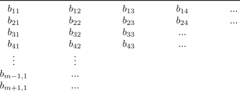
[image:2.595.297.541.726.820.2]

The table for numerator and denominator are derived according to Eq. 5 and is mentioned in Table 3 and Table 4.

Table 3. Routh stability array for numerator

b11 b12 b13 b14 ...

b21 b22 b23 b24 ...

b31 b32 b33 ...

b41 b42 b43 ...

..

. ...

bm−1,1 ...

(3)

[image:3.595.55.299.112.209.2]

Table 4. Routh stability array for denominator

a11 a12 a13 a14 ...

a21 a22 a23 a24 ...

a31 a32 a33 ...

a41 a42 a43 ...

..

. ...

an₋1,1 an₋1,2 ...

an,1 ...

The computed rows can be calculated by using follow-ing algorithm given as in Eq. 6.

cij =ci−2,j+2−

ci₋2,1.ci₋1,j+1

ci−1,1

(6) It holds for i ≥3 and i ≤ n−₂1+3. In RSA method, if the ﬁrst two rows known then the reduced model can be calculated by applying algorithm formula for computed rows. The transfer function forn−1 reduced system can be calculate by second generated row and ﬁrst computed rows as in Eq. 7.

Gn−1(s) =

b21s(m−1)+b31s(m−2)+b22s(m−3)+· · ·

a21s(m−1)+a31s(m−2)+a22s(m−3)+· · ·

(7) The reduced model of required order as 2nd_{, 3}rd_, _{· · ·}_,

etc. by applying this general formula applied which is given as in Eq. 8.

Rk(s) =

bm+2−k,0s(k−1)+bm+3−k,1s(k−2)+· · ·

an+1₋k,1sk+an+2₋k,1s(k−1)+· · ·

(8)

4 Stability equation method

In this method, a general phenomenon is used to con-struct reduced model of 2nd _{or 3}rd _{order from given in}

high order system. Stability equation method is based on elimination of high order terms in each step. Let consider a transfer function havingnthorder high order polynomial function which is given below in Eq. 9.

G(s) =bms

m₊_b

(m−1)s(m−1)+...+b1s+b0

ansn+a(n₋1)s(n−1)+...+a1s+a0

(9)

G(s) =N(s)

D(s) (10)

where, n≥m. In Eq. 10, N(s) and D(s) are the nu-merator, denominator part respectively. Each numera-tor and denominanumera-tor portion divided into two parts as even and another is odd. The numerator can be repre-sented in even and odd terms asN(s) =Ne(s) +No(s)

and the denominator can be represented as D(s) = De(s) +Do(s). Therefore, theG(s) can be written as in

Eq. 11.

G(s) = Ne(s) +N0(s) De(s) +Do(s)

(11) The even and odd terms of the polynomial are written as in Eq. 12 and Eq. 13. where,

Ne(s) = m ∑

i=0,2,4

bisi (12)

No(s) = m ∑

i=1,3,5

bisi (13)

These two equations are known as stability equation of N(s) andD(s). In this method, we reduce a high order polynomial system by successively discarding the least signiﬁcant factors from N(s) as well as D(s). In each step some unwanted or least signiﬁcant terms are elim-inated which can be understood by using mathematical explanation given below from Eq. 14 - 23.

D(s) =De(s)+Do(s) (14)

The expression for even and odd parts of the denomina-tor can be written as in Eq. 15 and Eq. 16.

De(s) =ao+ a2s2+ a4s4+· · · (15)

Do(s) =a1+ a3s3+ a5s5+· · · (16)

These may be written as

De(s) =ao k1

∏

i=1

(1 + s

2

zi2

) (17)

Do(s) =a1s k2

∏

i=1

(1 + s

2

pi2

) (18)

Wherek1andk2are integer parts ofn/2 and (n−2)/2,

respectively andz12< p12< z22< p22by discarding the

factors with larger magnitude of zi andpi, the reduced

stability equations of desired orderr become as Der(s) =ao

r1

∏

i=1

(1 + s

2

zi2

) (19)

Dor(s) =a1 r2

∏

i=1

(1 + s

2

pi2

) (20)

where, r1 and r2 are the integer parts of r/2 and (r−

1)/2, respectively. The reduced denominator of formed as

Dr(s) =Der(s) + Dor(s) (21)

The numerator is reduced similarly and we obtain Nr(s) =Ner(s) + Nor(s) (22)

The reduced orderR(s) is given by R(s) = Ner(s) +Nor(s)

Dor(s) +Der(s)

(23)

5 Illustrative Examples

(4)

[image:4.595.293.544.113.163.2]

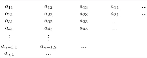
Table 5. Reduced models in literature for system in Example-1 [28]

S. No. Method 2ndorder reduced model

1 Desai, 2013 [29] 0.7645s+1.689

s2₊₂_.₅₉₁_s₊₁_.₆₈₉

2 Pati, 2014 [30] _s2₊₂₇s_.+24₀₀₉₆.0096_s₊₂₄_.₀₀₉₆

3 Desai, 2013 [31] _s20₊₁.6965_.₄₂₈s+0_s₊₀.6858_.₆₈₅₈

4 Philip, 2010 [32] _s2₊₂0.9315_.₇₅₆₁₂s+1_s₊₁.6092_.₆₀₉₂

5 Parmar, 2007 [17] 0.7442575s+0.6991576

s2+1.45771s+0.6997

6 Chen, 1980 [11] _s2₊₁0_..₄₅₇₇₁6997(_ss+1)₊₀_.₆₉₉₇

7 Parmar, 2007 [33] 0.6349s+4

s2₊₅_s₊₄

8 Mukherji, 1987 [28] 0.8000003_s2₊₃_s₊₂s+2

9 Lucas, 1983 [34] 0_s.2833₊₃s_s+2₊₂

10 Howitt, 1990 [35] _s20₊₁.81796.64068s+0s+0.78411.78411

11 Howitt, 1990 [35] 0.76434s+1.69073

s2+2.59288s+1.69073

12 Shoji,1982 [36] 0.7273s+2.6497

s2+3.5975s+2.6497

13 Singh, 2004 [5] 0.764444s+1.688910

s2+2.590980s+1.688910

14 Parmar, 2007 [37] 0.6667s+4

s2₊₅_s₊₄

15 Komarasamy, 2011 [15] _s2₊₃0._.8₀₀₀₄s+2_s.0004₊₂_.₀₀₀₄

16 Singh, 2012 [38] _s22₊₄.1931_.₇₆₁₈s+4_s₊₄.5714_.₅₇₁₃

17 Agrawal, 2011 [39] _s20₊₃.74791_.₇₆₉₂s+2_s₊₂.7692_.₇₆₉₂

18 Vishwakarma, 2008 [40] −0.189762s+4.5713

s2+4.76187s+4.5713

20 Panda, 2009 [41] 2.9319s+7.8849

3.8849s2+11.4839s+7.8849

21 Panda, 2009 [41] 5.2054s+8.989

[image:4.595.43.289.122.424.2]

3.8849s2+11.4839s+7.8849

Table 6. Denominator array using Routh stability array method

s4 ₁ ₃₅ ₂₄

s3 10 50 0

s2 ₃₀ ₂₄

s1 42 0

s0 ₂₄

5.1 Example-1

A fourth order SISO system is considered as presented in Eq. 24 [28].

G4(s) =

s3_{+ 7s}2_{+ 24s}_{+ 24}

s4_{+ 10s}3_{+ 35s}2_{+ 50s}_{+ 24} (24)

5.1.1 ROM in literature

The authors have screened the literature for second order reduced models using diﬀerent techniques of the system. The reduced models reported in literature are summarized in Table 5.

5.1.2 Proposed RSA based ROM

The RSA method applied on given problem shown in Eq. 24, on the basis of Routh stability array for both denominator in Table 6 and numerator in Table 7 com-puted terms gives the result as shown in Eq. 25.

R2(s) =

20.57143s+ 24

[image:4.595.41.289.457.517.2]

30s2_{+ 42s}_{+ 24} (25)

Table 7. Numerator array using Routh stability array method

s3 ₁ ₂₄

s2 7 24

s1 _20.57143 ₀

s0 24

5.1.3 Proposed hybrid RSA and SE based ROM

The prposed method includes use of Routh stabil-ity array method for numerator and stabilstabil-ity equation method determine the reduced order model. The RSA is used for reduced numerator and SE for reduced de-nominator. The numerator using RSA is given by Eq. 26 and the denominator using stability equation method is shown in Eq. 27. The reduced second order reduced model is given as in Eq. 28.

Nr(s) = 20.57143s+ 24 (26)

Dr(s) = 35s2+ 50s+ 24 (27)

R2(s) =

Nr(S)

Dr(S)

= 20.57143s+ 24

35s2_{+ 50s}_{+ 24} (28)

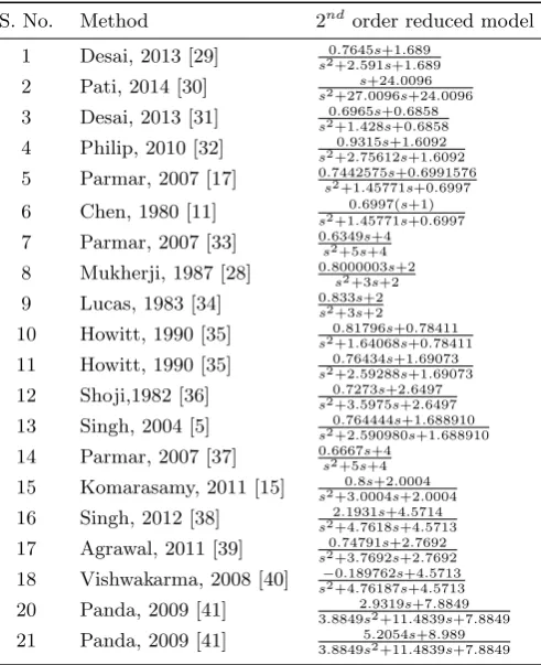
5.1.4 Results and discussion

The step response of the original system (as in Eq. 24, reduced order model in literature (as in Table 5) and that of with proposed (as in Eq. 25 and Eq. 28) are compared in terms of rise-time, settling-time, peak-time and peak as enlisted in Table 8. The step response of these systems are compared in Fig. 1 Fig. 7.

0 2 4 6 8 10

0 0.2 0.4 0.6 0.8 1

Time (s)

Amplitude

(a) Example−1

Original

RSA−MOR: Proposed RSA−SE: Proposed GA−MOR: Desai, 2013 Conv−MOR: Pati, 2014 BBBC−MOR: Desai, 2013

Figure 1. Step response of original system [28], Proposed ROM using RSA (Eq. 25), Proposed ROM using RSA and SE (Eq. 28), MOR in literature such as GA-MOR [29], Conv-MOR [30] and BBBC-MOR [31]

[image:4.595.307.526.497.667.2]

(5)

[image:5.595.60.551.111.398.2]

Table 8. Comapartive analysis of step response of original system, methods used in literature and proposed models for Example- I

Method Rise Settling Peak Peak

Time (s) Time (s) Time (s)

Original 2.2602 3.9307 6.9770 0.9991

Proposed RSA 1.9266 5.5869 4.0468 1.0359

Proposed RSA-SE 2.5389 3.7673 5.7285 1.0089

Desai, 2013 [29] 2.2616 3.8443 9.6778 1.0000

Pati, 2014 [30] 2.3875 4.2478 8.4934 0.9996

Desai, 2013 [31] 2.2716 3.3278 5.1430 1.0132

Philip, 2010 [32] 2.5288 4.5538 9.9334 0.9998

Parmar, 2007 [17] 2.1889 3.2202 4.9662 1.0122

Chen, 1980 [11] 2.3010 3.4111 5.2541 1.0107

Parmar, 2007 [33] 2.2694 4.0271 7.8163 0.9995

Mukherji, 1987 [28] 2.3413 4.0916 7.8163 0.9995

Lucas, 1983 [34] 2.3199 4.0643 7.8163 0.9995

Howitt, 1990 [35] 2.2550 3.5767 5.8832 1.0030

Howitt, 1990 [35] 2.2617 3.8449 9.6708 1.0000

Shoji,1982 [36] 2.2626 3.9618 7.5639 0.9995

Singh, 2004 [5] 2.2617 3.8446 9.6779 1.0000

Parmar, 2007 [37] 2.2645 4.0177 7.8163 0.9996

Komarasamy, 2011 [15] 2.3413 4.0915 7.8163 0.9995

Singh, 2012 [38] 1.3117 2.5404 4.3566 0.9983

Agrawal, 2011 [39] 2.2991 4.0453 7.8163 0.9995

Vishwakarma, 2008 [40] 1.8370 3.3411 5.7019 0.9991

Panda, 2009 [41] 2.2687 3.9175 7.2078 0.9994

Panda, 2009 [41] 1.9442 3.5022 6.7240 1.1393

0 2 4 6 8 10

0 0.2 0.4 0.6 0.8 1

Time (s)

Amplitude

(b) Example−1

Original

RSA−MOR: Proposed RSA−SE: Proposed BBBC−MOR: Philip, 2010 GA−MOR: Parmar, 2007 SE−MOR: Chen, 1980

Figure 2. Step response of original system [28], Proposed ROM using RSA (Eq. 25), Proposed ROM using RSA and SE (Eq. 28), MOR in literature such as BBBC-MOR [32], GA-MOR [17] and SE-MOR [11]

stability equation based SE-MOR [11], particle swarm optimization based PSO-MOR [18, 42], error minimiza-tion based EMT-MOR [28], factor division based FD-MOR [34, 37], integral square minimization based ISE-MOR [35, 5], iterative algorithm based Iter-ISE-MOR [36], PC-MOR [15, 38, 40], and clustering based Clus-MOR [39].

It could be easy to say that the proposed hybrid method based reduced order model is reﬂecting early settling to steady state as compared to original system and the RSA based reduced model. The peak value at-tained by the hybrid method based reduced model is

0 2 4 6 8 10

0 0.2 0.4 0.6 0.8 1

Time (s)

Amplitude

(c) Example−1

Original

RSA−MOR: Proposed RSA−SE: Proposed PSO−MOR: Parmar, 2007 EMT−MOR: Mukherjee, 1987 FD−MOR: Lucas, 1983

Figure 3. Step response of original system [28], Proposed ROM using RSA (Eq. 25), Proposed ROM using RSA and SE (Eq. 28), MOR in literature such as PSO-MOR [18], EMT-MOR [28] and FD-MOR [34]

lesser as compared to RSA and Original, as well.

5.2 Example-2

Considering another 4th order system as reported in [43] and presented in Eq. 29.

G4(s) =

4.269s3_{+ 5.10s}2_{+ 3.9672s}_{+ 0.9567}

4.39992s4_{+ 9.0635s}3_{+ 8.021s}2_{+ 5.362s}_{+ 1}

[image:5.595.323.541.428.604.2]

(6)

0 2 4 6 8 10 0

0.2 0.4 0.6 0.8 1

Time (s)

Amplitude

(d) Example−1

Original

[image:6.595.58.273.102.278.2]

RSA−MOR: Proposed RSA−SE: Proposed ISE−MOR: Howitt, 1990 ISE−MOR: Howitt, 1990 Iter−MOR: Shoji, 1982

Figure 4. Step response of original system [28], Proposed ROM using RSA (Eq. 25), Proposed ROM using RSA and SE (Eq. 28), MOR in literature such as ISE-MOR [35], ISE-MOR [35] and Iter-MOR [36]

0 2 4 6 8 10

0 0.2 0.4 0.6 0.8 1

Time (s)

Amplitude

(e) Example−1

Original

RSA−MOR: Proposed RSA−SE: Proposed ISE−MOR: Singh, 2004 FD−MOR: Parmar, 2007 PC−MOR: Komarasamy,2011

Figure 5. Step response of original system [28], Proposed ROM using RSA (Eq. 25), Proposed ROM using RSA and SE (Eq. 28), MOR in literature such as ISE-MOR [5], FD-MOR [37] and PC-MOR [15]

The 4th order original model of Eq. 29 is solved by diﬀerent researchers using diﬀerent techniques of reduc-tion, are summarized in Table 9.

5.2.2 Proposed RSA based MOR

The Routh stability array method is used to derive the 2nd _{order reduced model of the original system. To}

limit the size of paper, the steps of RSA technique are skipped and the reduced model is presented in Eq. 30.

R2(s) =

3.166386s+ 0.9567

5.417991s2_{+ 3.689147s}_{+ 1} (30)

5.2.3 Proposed hybrid RSA-SE based MOR

In this method, the numerator of reduced model is solved by RSA as in Eq. 30, while the denominator is

0 2 4 6 8 10

0 0.2 0.4 0.6 0.8 1

Time (s)

Amplitude

(f) Example−1

Original

[image:6.595.308.529.107.279.2]

RSA−MOR: Proposed RSA−SE: Proposed PC−MOR: Singh, 2012 Clus−MOR: Agarwal, 2011 CP−MOR: Vishwakarma, 2008

Figure 6. Step response of original system [28], Proposed ROM using RSA (Eq. 25), Proposed ROM using RSA and SE (Eq. 28), MOR in literature such as PC-MOR [38], Clus-MOR [39] and CP-MOR [40]

0 2 4 6 8 10

0 0.2 0.4 0.6 0.8 1

Time (s)

Amplitude

(g) Example−1

Original

RSA−MOR: Proposed RSA−SE: Proposed PSO−MOR: Panda, 2009 GA−MOR: Panda, 2009

Figure 7. Step response of original system [28], Proposed ROM using RSA (Eq. 25), Proposed ROM using RSA and SE (Eq. 28), MOR in literature such as PSO-MOR [41] and GA-MOR [41]

solved using SE method. The 2nd _{order reduced model}

is presented in Eq. 31. R2(s) =

3.166386s+ 0.9567

8.021s2_{+ 5.362s}_{+ 500} (31)

The original system of 4th_{order is reduced as in}

pre-vious sections. The step response of the original system of 4th_{order as in [43] and the reduced 2}nd_{order model}

in literature [45, 44] are compared with the proposed method based reduced models. The step response com-parison is shown in Fig. 8, and the respective step re-sponse information in terms of rise time, settling time, peak time and peak are enlisted in Table 10.

[image:6.595.56.273.352.523.2] [image:6.595.308.526.352.523.2]

(7)

[image:7.595.56.554.113.223.2]

Table 10. Comapartive analysis of step response of original system, methods used in literature and proposed models for Example-2

Original [43] 1.5621 9.0437 2.8939 0.9737

RSA-MOR: Proposed 2.1766 11.7025 5.3930 1.0882

RSA-SE: Proposed 4.5437 6.9973 11.4570 0.9650

ABC: Bansal, 2012 [44] 1.5768 2.8456 5.3816 0.9568

Pade: Bansal, 2012 [44] 3.1301 9.8472 18.6056 0.9543

Routh: Bansal, 2012 [44] 2.9087 4.3721 7.5517 0.9741

Aguirre, 1993 [45] 27.2242 48.8617 86.0420 0.4955

Table 9. The 2nd_{order reduced models in literature for}

Example-2

S. No. Method 2ndorder reduced model

1 ABC: Bansal,2012 [44] 0.2034s+8.9994

s2₊₇_.₉₂₄₉_s₊₉_.₄₀₀₈

2 Pade: Bansal,2012 [44] _s21₊₂.869_.₆₆₃s+0_s₊₀.5585_.₅₈₃₈

3 Routh: Bansal,2012 [44] _s02.₊₀6267_.₈₄₇s+0_s₊₀.1511_.₁₅₈

4 Aguirre, 1993 [45] _s20₊₁.2211_.₉₅₃₁s+0_s₊₀.0702_.₁₄₁₅

0 5 10 15 20

0 0.2 0.4 0.6 0.8 1

Time (s)

Amplitude

Example−2

Original

RSA−MOR: Proposed RSA−SE: Proposed ABC−MOR: Bansal, 2012 Pade−MOR: Bansal, 2012 RA−MOR: Bansal, 2012 Aguirre, 1993

Figure 8. Step response of original system [43], Proposed ROM using RSA, Proposed ROM using RSA and SE, MOR in litera-ture such as ABC-MOR [44], Pade-MOR [44], RA-MOR [44] and Aguirre-MOR [45]

5.3 Example-3

Considering another 5th _{order system as presented in}

Eq. 32 [46].

G(s) = 10s

4_{+ 82s}3_{+ 264s}2_{+ 396s}_{+ 156}

2s5_{+ 21s}4_{+ 84s}3_{+ 173s}2_{+ 148s}_{+ 40} (32)

The 5th _{order original model of Eq. 32 is solved by}

diﬀerent researchers using diﬀerent techniques of reduc-tion, are summarized in Table 11.

The Routh stability array method is used to derive the 2nd_{order reduced model of the original system [46].}

To limit the size of paper, the steps of RSA technique

are skipped and the reduced model is presented in Eq. 33.

R2(s) =

336.6974s+ 156

128.1566s2_{+ 123.1151s}_{+ 40} (33)

5.3.3 Proposed hybrid RSA-SE based MOR

In this method, the numerator of reduced model is solved by RSA as in Eq. 33, while the denominator is solved using SE method. The 2nd_{order reduced model}

is presented in Eq. 34. R2(s) =

336.6974s+ 156

173s2_{+ 148s}_{+ 40} (34)

The 5th order problem as in [46], the reduced mod-els in literature as shown in Table 11, and the proposed MOR using RSA and hybrid RSA-SE are compared sub-jected to step response. The step response comparison is shown in Fig. 9 and the step response information is compared in Table 12. It is found that the proposed method is able to retain original characteristics of the system even with 2nd _{order reduced model. The rise}

time with RSA is 2.3065 seconds while that of with orig-inal is 2.7457 seconds. The peak time with RSA and RSA-SE are 5.3515 seconds and 7.8459 seconds, respec-tively and reported as lower as compared to 10.4393 sec-onds with original system. It is again found the RSA-SE method based reduced order is able to quickly settle to steady state with minimum peak as compared to RSA model and the original system.

5.4 Example-4

Considering the 6th _{order multi-input multi-output}

(MIMO) system as presented in [37, 17]. It is two-input two-output system shown in following Eq. 35.

G(s) =

[ ₂₍_s₊₅₎ (s+1)(s+10)

(s+4) (s+2)(s+5) (s+10)

(s+1)(s+20)

(s+6) (s+2)(s+3)

]

(35)

The common denominator of Eq. 35 is represented by D(s) and presented in Eq. 36.

D(s) =s6+41s5+571s4+3491s3+10060s2+13100s+6000 (36) The numerator polynomials are mentioned in Eq. 37 -40.

[image:7.595.62.289.275.547.2]

(8)

[image:8.595.42.541.113.192.2]

Table 11. The 2nd_{order reduced models in literature for Example-3}

S. No. Method 2nd_{order reduced model}

1 PSO-MOR: Panda, 2009 [46] 347.0245s+225.6039

135.6805s2+166.3810s+57.8472

2 Conv.-MOR: Panda, 2009 [46] 369s+156

239.5s2+148s+40

3 DE-MOR: Yadav, 2011 [47] 369s+156

93.5606s2+151.1163s+39.890

4 Hwang,1996 [48] 2.487s+3.9

[image:8.595.41.539.223.332.2]

0.4951s2₊₁_.₈₃₈_s₊₁

Table 12. Step response information original system, proposed reduced models and the reduced models in literature for example-3

Original [46] 2.7457 5.4346 10.4393 3.8944

RSA: Proposed 2.3065 8.5242 5.3515 4.0888

RSA-SE: Proposed 3.4069 4.9892 7.8459 3.9643

PSO: Panda, 2009 [46] 2.9001 4.6323 7.7002 3.9120

Conv: Panda, 2009 [46] 3.3484 12.4151 7.3006 4.1744

DE: Yadav, 2011 [47] 3.3494 8.0352 17.1344 3.9070

Hwang,1996 [48] 2.9337 5.4490 9.4668 3.8945

0 5 10 15 20

0 0.5 1 1.5 2 2.5 3 3.5 4 4.5

Time (s)

Amplitude

Example−3

Original

RSA−MOR: Proposed RSA−SE: Proposed PSO−MOR: Panda, 2009 Conv−MOR: Panda, 2009 DE−MOR: Yadav, 2011 Iter−MOR: Hwang, 1996

Figure 9. Step response of original system [46], Proposed ROM using RSA, Proposed ROM using RSA and SE, MOR in litera-ture such as PSO-MOR [46], Conv.-MOR [46], DE-MOR [47] and Hwang-MOR [48]

N12(s) =s5+38s4+459s3+2182s2+4160s+2400 (38)

N21(s) =s5+30s4+331s3+1650s2+3700s+3000 (39)

N22(s) =s5+42s4+601s3+3660s2+9100s+6000 (40)

Therefore, the original four transfer functions are repre-sented byGij =Nij/Dij. These transfer functions are

associated to 2-inputs and 2-outputs.

The above original denominator of the 6thorder sys-tem as shown in Eq. 36 is subjected to reduce its 2nd order reduced polynomial. Similarly, the four numera-tor polynomials as shown in Eq. 37 - 40, are subjected to reduce to 2nd _{order transfer function. These are}

re-duced by diﬀerent researchers using diﬀerent techniques and are summarized in Table 13.

The 6th _{order original model of Eq. 35 is solved by}

Routh stability array method for denominator as well as for four-numerators. The 2nd_{order reduced model is}

shown in Eq. 41 and the associated four-numerators are shown in Eq. 42.

Dr(s) = 7448.008s2+ 10443.55s+ 6000 (41)

Nr11(s) = 6121.824s+ 6000

Nr12(s) = 3559.712s+ 2400

Nr21(s) = 2942.176s+ 3000

Nr22(s) = 7904.117s+ 6000

(42)

5.4.3 Proposed hybrid RSA- SE based MOR

The original systems denominator is reduced using stability equation method while the four numerators are reduced using Routh stability array method as in Eq. 42. The reduced 2nd order polynomials are shown in Eq. 43 and the transfer functions are shown in Eq. 44.

Dr(s) = 10060s2+ 13100s+ 6000 (43)

Gr11(s) = ₁₀₀₆₀6121_s2.₊₁₃₁₀₀824s+6000_s₊₆₀₀₀

Gr12(s) = 100603559s2.+13100712s+2400s+6000

Gr21(s) = ₁₀₀₆₀2942_s2.₊₁₃₁₀₀176s+3000_s₊₆₀₀₀

Gr11(s) = ₁₀₀₆₀7904_s2.₊₁₃₁₀₀117s+6000_s₊₆₀₀₀

(44)

In this section, the system with inputs and two-outputs is considered. It results to four transfer func-tions. These transfer functions are denoted by Gij(s)

and to be analysized separately. The comparative re-sponse of original system, reduced models in literature and the proposed models asG11(s),G12(s),G21(s) and

[image:8.595.55.270.361.536.2]

(9)

[image:9.595.56.555.110.409.2]

Table 13. The 2nd_{order reduced models in literature for Example-4}

S. No. Method Reduced order model

1 Parmar, 2007 [37]

Dr(s) =s2+ 13.6666s+ 8.4707

r11(s) = 6.0429s+ 8.4707

r12(s) = 3.9419s+ 3.3883

r21(s) = 2.8097s+ 4.2354

r22(s) = 8.0195s+ 8.4707

2 Parmar, 2007 [17]

Dr(s) =s2+ 1.34952s+ 0.6181 r11(s) = 0.8503087s+ 0.6171331

r12(s) = 0.4617562s+ 0.2466069

r21(s) = 0.4093304s+ 0.3086095

r22(s) = 0.9976611s+ 0.6171125

3 Komarasamy, 2011 [15]

Dr(s) =s2+ 4.0847s+ 3.0847

r11(s) = 1.30487s+ 3.0847

r12(s) = 1.0786s+ 1.23388

r21(s) = 0.5771s+ 1.54235

r22(s) = 2.0282s+ 3.0847

4 Vishwakarma, 2009 [49]

Dr(s) =s2+ 4.3374s+ 3.65079 r11(s) = 1.18156s+ 3.65079

r12(s) = 1.04664s+ 1.46031

r21(s) = 0.49819s+ 1.82539

r22(s) = 1.6911s+ 3.65079

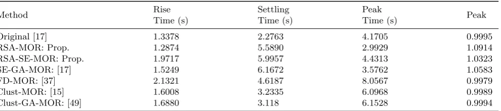
the response data is compared in Table 14 Table 17. The response due to proposed models and that of with original systems are as quite similar in terms of rise time, settling time, peak time and peak. It is also compara-tive to the systems reduced in literature using diﬀerent control techniques as presented in [37, 17, 15, 49].

0 5 10 15

0 0.2 0.4 0.6 0.8 1

Time (s)

Amplitude

(a) R₁₁(s): Example−4

Original

[image:9.595.69.286.527.700.2]

RSA−MOR: Proposed RSA−SE: Proposed SE−GA−MOR: Parmar, 2007 FD−MOR: Parmar, 2007 Clus−MOR: Komarasamy, 2011 Clus−GA−MOR: Vishwakarma, 2009

Figure 10. Step response for G11(s) of original system [17],

Proposed ROM using RSA, Proposed ROM using RSA and SE, MOR in literature such as [17, 37, 15, 49]

The rise time associated to 2nd order reduced model using proposed RSA is 1.6712 seconds, which is lower as compared to original G11(s) and its reduced

mod-els in literature. Similarly, for G21(s) and G22(s); the

rise time is again lower as 1.7286 and 1.2874 seconds respectively and found to be lesser as compared to

orig-0 5 10 15

0 0.05 0.1 0.15 0.2 0.25 0.3 0.35 0.4 0.45 0.5

Time (s)

Amplitude

(b) R₁₂(s): Example−4

Original

Figure 11. Step response forG12(s) of original system [17],

inal and reduced models in literature. It is again estab-lished while considering the multivariable system that the model with RSA-SE is able to quickly settle as com-pared to RSA-MOR and original system.

6 Conclusion

(10)

[image:10.595.53.539.141.251.2]

Table 14. Comparative analysis of step response of original system, methods used in literature and proposed method of system of Example -4 forG11(s)

Original [17] 2.1254 3.7944 8.5950 0.9998

RSA-MOR: Prop. 1.6712 5.5839 3.5915 1.0502

RSA-SE-MOR: Prop. 2.4575 3.5435 5.3982 1.0161

SE-GA-MOR: [17] 1.8627 5.8176 4.1982 1.0312

FD-MOR: [37] 2.6393 5.1309 9.4531 0.9988

Clust-MOR: [15] 2.0639 3.7543 7.2917 0.9994

[image:10.595.46.538.326.436.2]

Clust-GA-MOR: [49] 1.9093 3.4067 6.8396 0.9996

Original [17] 1.0216 1.8653 3.6459 0.3998

RSA-MOR: Prop. 1.1152 5.5910 2.6936 0.4495

RSA-SE-MOR: Prop. 1.7248 6.2178 3.9479 0.4193

SE-GA-MOR: [17] 1.2438 6.3842 3.0320 0.4394

FD-MOR: [37] 1.4314 3.9153 9.1852 0.3997

Clust-MOR: [15] 0.9931 2.2690 7.8058 0.4000

Clust-GA-MOR: [49] 1.0691 2.3330 3.9246 0.3987

Original [17] 2.1808 3.8582 8.8500 0.4999

RSA-MOR: Prop. 1.7286 5.5829 3.7412 0.5232

RSA-SE-MOR: Prop. 2.5221 3.6481 5.5593 0.5074

SE-GA-MOR: [17] 1.9439 5.6955 4.3537 0.5135

FD-MOR: [37] 2.7284 5.2215 8.7117 0.4990

Clust-MOR: [15] 2.1342 3.8353 8.3409 0.4999

Clust-GA-MOR: [49] 1.9702 3.4836 6.8396 0.4998

Original [17] 1.3378 2.2763 4.1705 0.9995

RSA-MOR: Prop. 1.2874 5.5890 2.9929 1.0914

RSA-SE-MOR: Prop. 1.9717 5.9957 4.4313 1.0323

SE-GA-MOR: [17] 1.5249 6.1672 3.5762 1.0583

FD-MOR: [37] 2.1321 4.6187 8.0567 0.9979

Clust-MOR: [15] 1.6008 3.2335 6.0968 0.9989

[image:10.595.44.542.510.619.2] [image:10.595.46.541.693.803.2]

(11)

0 5 10 15 0

0.1 0.2 0.3 0.4 0.5

Time (s)

Amplitude

(c) R₂₁(s): Example−4

Original

[image:11.595.70.289.104.279.2]

0 5 10 15

0 0.2 0.4 0.6 0.8 1

Time (s)

Amplitude

(d) R₂₂(s): Example−4

Original

array (RSA) method and (ii) the combination of RSA and stability equation (SE) method. The systems re-duced order models in literature are considered to com-pare the response due to proposed RSA based model and proposed RSA-SE based model. The original sys-tems, the respective reduced models of the systems and proposed reduced order models are subjected to step re-sponse and its information in terms of rise time, settling time, peak time and peak. The graphical and statistical comparative analysis have been carried out and found to be satisfactory response as compared to original system and reduced models in literature.

REFERENCES

[1] D. K. Sambariya and H. Manohar, “Model order reduc-tion by integral squared error minimizareduc-tion using bat algorithm,” inIEEE Proceedings of 2015 RAECS UIET Panjab University Chandigarh21−22ndDecember 2015, 2015, pp. 1–7.

[2] D. K. Sambariya and H. Manohar, “Preservation

of stability for reduced order model of large scale systems using diﬀerentiation method,” British Journal of Mathematics & Computer Science, vol. 13, no. 6, pp. 1–17, 2016. [Online]. Available: http://dx.doi.org/10. 9734/BJMCS/2016/23082

[3] H. Manohar and D. K. Sambariya, “Model order reduc-tion of mimo system using diﬀerentiareduc-tion method,” in

IEEE Proceeding of 10th _{International Conference on}

Intelligent Systems and Control (ISCO 2016), vol. 2, 2016, pp. 347–351.

[4] D. K. Sambariya and H. Manohar, “Model order re-duction by diﬀerentiation equation method using with routh array method,” inIEEE Proceeding of10th Inter-national Conference on Intelligent Systems and Control (ISCO 2016), vol. 2, 2016, pp. 341–346.

[5] V. Singh, D. Chandra, and H. Kar, “Optimal routh approximants through integral squared error minimi-sation: computer-aided approach,” IEE Proceedings -Control Theory and Applications, vol. 151, no. 1, pp. 53–58, Jan 2004. [Online]. Available: http://dx.doi. org/10.1049/ip-cta:20040007

[6] I. El-Nahas, N. Sinha, and R. Alden, “Pade and routh approximation in the time domain,” in Decision and Control, 1983. The 22nd IEEE Conference on, Dec 1983, pp. 243–246. [Online]. Available: http://dx.doi. org/10.1109/CDC.1983.269837

[7] H. N. Soloklo and M. M. Farsangi, “Multiobjective weighted sum approach model reduction by routh-pade

approximation using harmony search,” Turk J Elec

Eng & Comp Sci, vol. 21, no. 0, pp. 2283 – 2293, 2013. [Online]. Available: http//dx.doi.org/10.3906/ elk-1112-31

[8] V. Singh, “Obtaining routh-pade approximants using the luus-jaakola algorithm,” IEE Proceedings - Control Theory and Applications, vol. 152, no. 2, pp. 129–132, March 2005. [Online]. Available: http://dx.doi.org/10. 1049/ip-cta:20041305

[9] D. K. Sambariya and G. Arvind, “High order diminution of LTI system using stability equation method,”British Journal of Mathematics & Computer Science, vol. 13, no. 5, pp. 1–15, 2016. [Online]. Available: http://dx. doi.org/10.9734/BJMCS/2016/23243

[10] D. K. Sambariya and R. Prasad, “Routh stability ar-ray method based reduced model of single machine inﬁ-nite bus with power system stabilizer,” inInternational Conference on Emerging Trends in Electrical, Commu-nication and Information Technologies (ICECIT-2012), 2012, pp. 27–34.

[11] T. C. Chen, C. Y. Chang, and K. W. Han,

“Model reduction using the stability-equation method and the continued-fraction method,” International Journal of Control, vol. 32, no. 1, pp. 81–94, 1980. [Online]. Available: http://dx.doi.org/10.1080/ 00207178008922845

[12] D. K. Sambariya and G. Arvind, “Reduced order mod-elling of SMIB power system using stability equation

method and ﬁreﬂy algorithm,” in 6th IEEE

Inter-national Conference on Power Systems, (ICPS-2016), 2016, pp. 1–6.

[13] D. K. Sambariya and R. Prasad, “Diﬀerentiation

[image:11.595.69.287.339.513.2]

(12)

International Journal of Applied Engineering Research,

vol. 7, no. 11, pp. 2116 – 2120, 2012.

[On-line]. Available: http://gimt.edu.in/clientFiles/FILE REPO/2012/NOV/24/1353741189722/202.pdf.

[14] D. K. Sambariya and A. S. Rajawat, “Application of routh stability array method to reduce MIMO SMIB power system,” in6th IEEE International Conference on Power Systems, (ICPS-2016), 2016, pp. 1–6.

[15] R. Komarasamy, N. Albhonso, and G. Gurusamy, “Order reduction of linear systems with an improved pole clustering,” Journal of Vibration and Control, vol. 18, no. 12, p. 18761885, 2011. [Online]. Available: http://dx.doi.org/10.1177/1077546311426592

[16] H. N. Soloklo, O. Nali, and M. M. Farsangi, “Model re-duction by hermite polynomials and genetic algorithm,”

Journal of mathematics and computer science, vol. 9, no. 0, pp. 188–202, 2014.

[17] G. Parmar, S. Mukherjee, and R. Prasad, “Order re-duction of linear dynamic systems using stability equa-tion method and ga,” International Journal of Com-puter, Information, and Systems Science, and Engineer-ing, vol. 1, no. 2, pp. 26–32, 2007.

[18] G. Parmar, S. Mukherjee, and R. Prasad, “Reduced order modeling of linear dynamic systems using parti-cle swarm optimized eigen spectrum analysis,” Interna-tional Journal of ComputaInterna-tional and Mathematical Sci-ence, vol. 1, no. 1, pp. 45–52, 2007.

[19] A. Sikander and R. Prasad, “Soft computing approach for model order reduction of linear time invariant systems,” Circuits, Systems, and Signal Processing, vol. 34, no. 11, pp. 3471–3487, 2015. [Online]. Available: http://dx.doi.org/10.1007/s00034-015-0018-4

[20] D. K. Sambariya and R. Prasad, “Routh approximation based stable reduced model of single machine inﬁnite bus system with power system stabilizer,” in DRDO-CSIR Sponsered: IX Control Instrumentation System Conference (CISCON - 2012), 2012, pp. 85–93.

[21] D. K. Sambariya and R. Prasad, “Stable reduced model of a single machine inﬁnite bus power system with power system stabilizer,” inInternational Conference on Advances in Technology and Engineering (ICATE’13), Jan 2013, pp. 1–10. [Online]. Available: http://dx.doi. org/10.1109/ICAdTE.2013.6524762

[22] D. K. Sambariya and R. Prasad, “Stability equation method based stable reduced model of single machine inﬁnite bus system with power system stabilizer,” In-ternational Journal of Electronic and Electrical Engi-neering, vol. 5, no. 2, pp. 101–106, 2012.

[23] D. K. Sambariya and R. Prasad, “Stable reduced model of a single machine inﬁnite bus power system,” in

17th National Power Systems Conference (NPSC-2012), 2012, pp. 541–548.

[24] D. K. Sambariya and O. Sharma, “Model order

reduction using routh approximation and cuckoo search algorithm,”Journal of Automation and Control, vol. 4, no. 1, pp. 1–9, 2016. [Online]. Available: http://pubs. sciepub.com/automation/4/1/1

[25] D. K. Sambariya and G. Arvind, “Reduced order model of single machine inﬁnite bus power system using stability equation method and self-adaptive bat algo-rithm,”Universal Journal of Control and Automation, vol. 4, no. 1, pp. 1–7, 2016. [Online]. Available: http:// dx.doi.org/10.13189/ujca.2016.040101

[26] D. K. Sambariya and A. S. Rajawat, “Model order reduction of lti system using routh stability array method,” inIEEE proceedings on International Confer-ence on Computing, Communication and Automation (ICCCA-2016), 2016, pp. 1–6.

[27] V. Krishnamurthy and V. Seshadri, “Model reduction using the routh stability criterion,”Automatic Control, IEEE Transactions on, vol. 23, no. 4, pp. 729–731, Aug 1978. [Online]. Available: http://dx.doi.org/10.1109/ TAC.1978.1101805

[28] S. Mukherjee and R. Mishra, “Order reduction of linear systems using an error minimization technique,”

Journal of the Franklin Institute, vol. 323, no. 1, pp. 23 – 32, 1987. [Online]. Available: http://www.sciencedirect. com/science/article/pii/0016003287900378

[29] S. R. Desai and R. Prasad, “Implementation of

order reduction on tms320c54x processor using genetic

algorithm,” in Emerging Research Areas and 2013

International Conference on Microelectronics, Commu-nications and Renewable Energy (AICERA/ICMiCR), 2013, pp. 1–6. [Online]. Available: http://dx.doi.org/ 10.1109/AICERA-ICMiCR.2013.6576027

[30] A. Pati, A. Kumar, and D. Chandra, “Suboptimal control using model order reduction,”Chinese Journal of Engineering, vol. 2014, p. 5, 2014. [Online]. Available: http://dx.doi.org/10.1155/2014/797581

[31] S. R. Desai and R. Prasad, “A new approach to order reduction using stability equation and big bang big crunch optimization,” Systems Science & Control Engineering, vol. 1, no. 1, pp. 20–27, 2013. [Online]. Available: http://dx.doi.org/10.1080/21642583.2013. 804463

[32] B. Philip and J. Pal, “An evolutionary computation

based approach for reduced order modelling of

linear systems,” in IEEE International Conference on Computational Intelligence and Computing Research (ICCIC ’10), 2010, pp. 1–8. [Online]. Available: http:// dx.doi.org/10.1109/iccic.2010.5705729

[33] G. Parmar, S. Mukherjee, and R. Prasad, “Reduced order modeling of linear dynamic systems using parti-cle swarm optimized eigen spectrum analysis,” Interna-tional Journal of ComputaInterna-tional and Mathematical Sci-ence, vol. 1, no. 1, pp. 45–52, 2007.

[34] T. Lucas, “Factor division: a useful algorithm in model reduction,” IEE Proceedings D - Control Theory and Applications, vol. 130, no. 6, pp. 362–364, November 1983. [Online]. Available: http://dx.doi.org/10.1049/ ip-d.1983.0060

[35] G. D. Howitt and R. Luus, “Model reduction by minimization of integral square error performance indices,” Journal of the Franklin Institute, vol. 327, no. 3, pp. 343 – 357, 1990. [Online]. Avail-able: http://www.sciencedirect.com/science/article/ pii/001600329090001Y

[36] F. Shoji, “Comments on simpliﬁcation of large linear systems using a step iterative method: A two-step projection algorithm,” Journal of the Franklin Institute, vol. 313, no. 5, pp. 267 – 271, 1982. [Online]. Available: http://www.sciencedirect.com/ science/article/pii/0016003282900023

(13)

vol. 31, no. 11, pp. 2542 – 2552, 2007. [Online]. Avail-able: http://www.sciencedirect.com/science/article/ pii/S0307904X06002411

[38] V. P. Singh, P. Chaubey, and D. Chandra, “Model order reduction of continuous time systems using pole clustering and chebyshev polynomials,” in Students Conference on Engineering and Systems (SCES-12), 2012, pp. 1–4. [Online]. Available: http://dx.doi.org/ 10.1109/sces.2012.6199028

[39] S. K. Agrawal, D. Chandra, and I. A. Khan, “Order reduction of linear system using clustering, integral square minimization and dominant pole technique,”

International Journal of Engineering and Technology, vol. 3, no. 1, pp. 64–67, 2011. [Online]. Available: http://dx.doi.org/10.7763/IJET.2011.V3.201

[40] C. B. Vishwakarma and R. Prasad, “Clustering method for reducing order of linear system using pade approx-imation,” IETE Journal of Research, vol. 54, no. 5, pp. 326–330, 2008. [Online]. Available: http://www. tandfonline.com/doi/abs/10.4103/0377-2063.48531

[41] S. Panda, J. S. Yadav, N. P. Patidar, and C. Ardil, “Evo-lutionary techniques for model order reduction of large scale linear systems,” International Journal of Applied Science, Engineering and Technology, vol. 5, no. 1, pp. 22–28, 2009.

[42] S. Panda, S. K. Tomar, R. Prasad, and C. Ardil, “Re-duction of linear time-invariant systems using routh-approximation and pso,”International Journal of Elec-trical, Robotics, Electronics and Communications Engi-neering, vol. 3, no. 9, pp. 20–27, 2009.

[43] L. A. Aguirre, “The least squares pad method for model reduction,” International Journal of Systems Science, vol. 23, no. 10, pp. 1559–1570, 1992. [Online]. Available: http://dx.doi.org/10.1080/00207729208949408

[44] J. Bansal, H. Sharma, and K. Arya, “Model order reduction of single input single output systems us-ing artiﬁcial bee colony optimization algorithm,” in

Nature Inspired Cooperative Strategies for Optimiza-tion (NICSO 2011), ser. Studies in Computational Intelligence, D. Pelta, N. Krasnogor, D. Dumitrescu, C. Chira, and R. Lung, Eds. Springer Berlin Heidel-berg, 2011, vol. 387, pp. 85–100. [Online]. Available: http://dx.doi.org/10.1007/978-3-642-24094-2 6

[45] L. Aguirre, “Validation of reduced-order models for closed loop applications,” in Control Applications, 1993., Second IEEE Conference on, Sep 1993, pp. 605–610 vol.2. [Online]. Available: http://dx.doi.org/ 10.1109/CCA.1993.348337

[46] S. Panda, S. K. Tomar, R. Prasad, and C. Ardil, “Model reduction of linear systems by conventional and evolu-tionary techniques,”International Journal of Electrical, Robotics, Electronics and Communications Engineering, vol. 3, no. 11, pp. 29–34, 2009.

[47] J. S. Yadav, N. P. Patidar, J. Singhai, S. Panda, and C. Ardil, “A combined conventional and diﬀerential evo-lution method for model order reduction,”International Journal of Electrical, Robotics, Electronics and Commu-nications Engineering, vol. 5, no. 9, pp. 68–75, 2011.

[48] C. Hwang and J.-H. Hwang, “A new two-step iterative method for optimal reduction of linear siso systems,”

Journal of the Franklin Institute, vol. 333, no. 5, pp. 631–645, 1996.