Environments Aware for Prolonging the Lifetime of
Sensor Nodes Deployed in WSNs
Joy Iong-Zong Chen1, Lu-Tsou Yeh2
1Department of Electrical Engineering, Dayeh University, Changhwa, Chinese Taipei 2Department of Electrical Engineering, Asia-Pacific Institute of Creativity,
Miaoli, Chinese Taipei Email: [email protected]
Received November 14, 2011; revised December 12, 2011; accepted December 18, 2011
ABSTRACT
Providing a pretty adequate environment condition between the transmission and the receiver for a WSN (wireless sen-sor network), in which deployed sensen-sor nodes and fusion center, is investigated in the paper. Moreover, an algorithm promotes the energy efficient, increases the accuracy of sensing data and prolongs the lifetime of sensor nodes deployed over an WSNs is proposed. On the basis of adopting sensor management, which involves sensor movement sequences, sensor location arrangement, lifetime requirement for sensor nodes deploy surveillance environment, and the data fu-sion center, are addressed too. Simulation results from the lifetime performance for sensor nodes defeated by parame-ters about the environment around the WSNs are illustrated. Parameparame-ters aforementioned are including sensing distance, path loss factor, number bits of a transmitted packet, and interference suffering from the path of data transmission etc. Furthermore, the algorithm of sensor location arrangement is modified for the purpose of improving the lifetime per-formance in WSNs environments. In addition, simulation results show that the proposed algorithm in this paper is not only definitely to improve the energy efficient sufficiently, but the sensing accuracy and the lifetime performance of the sensor nodes are also prolonged significantly.
Keywords: Lifetime; Path Loss Factor; Sensor Movement Sequence; Sensor Location Arrangement; WSNs (Wireless Sensor Networks)
1. Introduction
Recently, the advantages of WSNs (wireless sensor net-work) has fast grown for applying to, such as, military surveillance, health caring, planet monitoring, and a lot of other kinds of relative fields. One of the most impor-tant reasons for lasting all the application of WSNs is the support of energy to each sensor nodes distributed in the sensing areas. Therefore, the schemes of concerting for prolonging the lifetime of sensor nodes become remark-able issues to discuss. According to the protocol of IEEE 802.15.4 [1], there are many factors that dominate the lifetime of sensor nodes which equipped with energy constrained battery. Hence, to the best of professional person’s knowledge, the evaluation of the survivability of sensor nodes in WSNs is critical concern in the de-signing of WSNs.
We proposed a scheme of adopting sensors location arrangement for the purpose of improving the lifetime performance of the WSNs scenario in this paper. It is known that the lifetime of every un-pre-located sensor will affect definitely the detection performance for WSNs. So far, there are several researches have been
increase WSN service time. In [7] researches assumed that a BS deployed in a mobile device, such as a vehicle, moving with a certain speed, causes the BS to be peri- odically re-deployed to varied positions in order to in- crease the lifetime of WSN. The scheme moving the lo- cation of a BS to areas with lower activity to redistribute WSN traffic flow is presented in [8]. The authors in [9] to maximize the lifetime of WSN with the algorithm which is designed a delay-tolerant application for mobile BS. Thus, the original routing paths will change with the change in BS location and the WSN will need to re-gen- erate new routing paths. In [10] authors presented a me- thod with adopting the mobility BS and avoiding the at- tack from the enemy for prolonging the WSN lifetime. Two autonomous moving schemes for the mobile sink are alleviated in [11] in which the sink makes moving decisions without complete knowledge of network to- pology and the energy distribution of all sensor nodes causes the WSN lifetime be prolonged. In [12] the per-formance evaluation is held in considering consumed energy metric for mobile sink with two cases: when the sink node is mobile and stationary considering lattice and random topologies using AODV protocol.
Motivated by the preview work results, In this paper some factors, such as sensing distance, path loss factor, number bits of a transmitted packet, interference suffer-ing from path of data transmission, are involved in the system performance analysis. An environment aware algorithm for promoting the energy efficient, increasing the accuracy of sensing data and prolonging the lifetime of sensor nodes for WSNs is proposed. The paper is or-ganized as follows, the scenario model related to WSNs is described in Section 2. The lifetime performance ana- lysis of WSNs is studied in Section 3. In Section 4 the results and discussion are illustrated. There is a brief conclusion is drawn in Section 5.
2. Scenarios Relate to WSNs
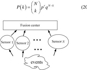
It is known that the realizable and the accuracy of sensed data gathered from the algorithm of decentralized proc- essing in WSNs is more believable than that of the cen- tralized processing, and the load of data transportation between each node can be reduced. In the paper a sensor network shown in Figure 1 is deployed with a fusion center (sensor C), the sensing distance (radius from the center) Rs, and the transmission distance c, where the
condition of
R
s c can makes not only sure that all of
the sensors without meeting the problem of existence of hole area, but they are also able to communicate with each other smoothly. Thereafter, the scenario of the WSNs shown in Figure 1 is a deployment with a local sensing fusion from N sensors. Before the analysis of
lifetime performance is illustrated, the requirement of
[image:2.595.345.489.81.212.2]R R
Figure 1. Diagram of local fusion of sensor data.
introducing to means of fusion among the sensor nodes is necessary. There two means of data fusion are included: 1) maximum number fusion, and 2) majority detection fusion. Basically, the fusion nodes are required to per- form event detection based on the maximum measure- ment number, such that the missing probability, P(M),
can be reduced. Consider that there is a maximum num- ber, s, selected from n sensed measurements i,
1,
i ,n, which is given as
1 2
max , , ,
s Arg n
(1)
where max
is the function of selecting the maximum one element, and the CDF (cumulate distribution func-tion) of the events’ random variable for the selection fact can be written as
s
1 , , n
P x P x x (2)
where the measured values on each of the nth sensor
node are considered independently each other. Hence, after the maximum value has been fused in the fusion center, the missing probability, P M , of a single sensor
node can be calculated as
( ) (1)
1 (1) (1) (
Pr
Pr ,
M S th
n
th n th m
P Hyp
)
Hyp Hyp P P
(3) where Hyp(1) represents the hypothesis that when the
event happens, m represent the probability occurs in
each event of fused sensor, and th indicated the detec-
tion threshold value. By the way, following up operation rule of the detection theory, after the maximum value is fused the detection probability, ( )
P
D
P , and false alarm
probability, P(FA), can be determined as
( )1 (1) (1)
( )
Pr
1 Pr , ,
1 1
D s th
th n th
n d
P Hyp
Hyp Hyp
P
( ) (0)
1 (0) (0)
( )
Pr
1 Pr , ,
1 1
FA s th
th n th
n fd P Hyp Hyp Hyp P
(5)
respectively. Then, the cost function of detection error probability, P( )E , can be given as
( )E 0 (FA) 1 (M)
P z P z P (6) where 1, and 0 are corresponding to express the pri- ori probabilities of event occurring and without occurring. Similarly, in the majority detection fusion, the false alarm probability, ( )
z z
fa , and the missing probability,
, can be expressed as P
( )m
P
( ) ( )
Pr 1 0 , and
Pr 0 1 ,
fa m
P y Hyp P y Hyp
(7)
respectively, where the random variable is used to make decision the states of an event occurring or without oc- curring. Thus, the detection probability, P( )d , is given as
( )d Pr 1 1 1 ( )m
P y Hyp P
m
m
(8)
and the detection error probability, , can be obtained
as ( )e
P
( )e 0 (fa) 1 ( )
P z P z P (9)
Once the detection probability and the error probabil- ity of the individual sensor node, accordingly, the fusion will be held immediately Basis on the condition that there are n events occur really from N sensor nodes, and
the total missing probability and the false alarm probabil- ity of the local fusion can be correspondingly expressed as
1 ( ) ( ) ( ) 1 1 ( ) ( ) ( ) 0 1 , 1 jn N n
M m
n j
N n n
FA fa fa
n
N
P P
n N
P P P
n
P (10)3. Lifetime Performance Analysis
In the paper three reasons are mentioned to analyze the lifetime performance of WSNs, though there are several parameters definitely control the lifetime performance, such as the sensing distance, the sensor numbers, and the fusion algorithm. The much most important reason should be the condition of transmission environments between the sensor node and the fusion center.
For a given event, e.g., the tracking of some targets, and assume that the WSNs is deployed in a squared area of size AreaLength Length , the total number of
sensor nodes is N, thus d N Area
ered as unifor
denotes the node
the following discussion. The discrete Poisson distribu- tion can be used to characterize the probability that there are g sensor nodes located within the area around the
event [13]. Within the WSN the probability with random variable g can be expressed as
exp
π 2
π 2
g ! d s d sP g R R g (11)
It should be claimed that the covered area of WSN will be
g (12)
In the case wherein the probability that any event is de
constrained avoiding the results from the simulation becomes divergent. In addition, by combining the previ- ous equation with (6) for the purpose of determining the average detection error probability, Perr, in fusion center,
it is obtained as
1 N err E
g
P P P
tected by at least g times within in sensor nodes can be
calculated as
1
2
20
0
π
d 1 exp π
!
s
g g
R d S
g g d
i
R
P f x x R
g
S (13)where Rs indicates the sensing range in which a target
can be detected, the pdf (probability density function),
g
f x , of the range counting from any node in WSNs to
nearest sensor node can be modeled as
its gth
2 1
2π g g 1 !exp π 2
g d d
f x x g x (14)
The most concerned event for lifetime perform W
ance of SNs should be the supporting energy which is include- ing both the transmission and the receive energies. The lifetime performance can be evaluated by defining how long the sensor node in the whole network to finish the duties involving data sensing and data fusion, that is, with N randomly deployed sensor nodes the sensing life-
time, LT, should be definitely defined as
0
T Eng (15)
where denotes the savable energy of a single sen-
L N E E
(0)
E
sor node,
represents the expectation operator, and the average e gy of each sensor can be written asN ner
1 11
Eng k
E P k k
E (16)
where P k
energ
is shown in (11), E(1) expresses the dis- de
sipated y of a single sensor no , and it can be cal- culated as
(1) 2 elec amp cp
E Bit E E r (17)
where p
epr
denotes the exponent path loss [8], Eelec and plete
amp
E r esents the power supported to com the
mission between transmitter and receiver of a fusion trans
sensor and the power for amplifying the transmitted sig- nal, respectively. There is also the parameter Bit which is
the transmission bit number of one packet, which sizes depend on what communication schemes were adopted,
i.e., the modulation schemes of the wireless communica-
tion will determine the size of Bit.
3.1. Transmission Bit Number and Path Loss
It is believed that lifetime of the sensor node will be
Factor
deeply overruled by the length of the transmission bit number, Bit. Additionally, conditions of propagation chan-
nel between sensing node and the fusion center are in- volved in this study. The exponent path loss is consid- ered as the parameter for evaluation the lifetime per- formance, and the path loss factor is given as [14]
rpp Rs (18) where p
sm
is the exponent path loss, then the length of the tran ission bit number can be easily obtained as
exp s
Bit R (19)
Furthermore, the fading situation m
3.2. Sensor Location Arrangement
one of them is
(20) of the wireless com- unication channel is taken into account the simulation model. The channel fading model is characterized by the Nakagami-m statistical distribution which is the most
useful one which is for experimental in accuracy. The severe fading of the channel situation is quantied with the fading figures, m. The larger value of m, the superior of
the communication channel is [15].
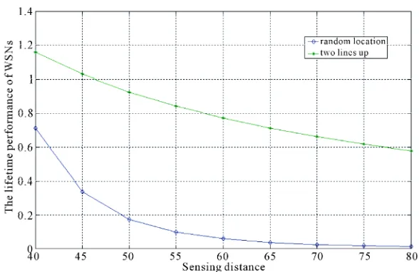
Two scenarios in the paper are proposed,
the random arrangement and the other one lines up ar- rangement of sensor nodes. The one shown in Figure 2 is the latter scenario in which the single sensor node as- sumed modeled as Poisson distribution. Consider the there are k sensors nodes selected from the total sensors
randomly, and its probability can be written as
N
r N kP k p q k
Figure 2. The scenario of local fusion from N nsors.
wh
se
ere p 1 q. Thereafter, with the assumption de-
previous
scribed ly that means there are g sensor nodes
are selected out from the N sensor nodes, and they can
transmit the sensing data to fusion center after the sens- ing operations sequence of the event is completed. Here- after, the error probability of detection under the case of that the sensor location arrangement with two lines up can be obtained by some random variables transform, and shown as
2 2 2π
π π
g N g
s err
s s
N R
P g
g R R
(21)
where and are both two parameters of the Pois-
sor node son statistical distribution.
4. Simulation Results and Discussion
Consider some factors for the lifetime of a sen
WSNs. For instance, the path loss factor, p, of the
transmission channel between the sensor no and the fusion center, the bit number, Bit, for transmitting the
sensed data to the fusion center, and the sensing range, de
s
R , etc. The area is considered as 1000 1000 square
the numerical results. The numbe nodes is
assumed as N 350
for r of sensor
for both the calculation of Figures
3 and 4. The rom comparing with different ex-
ponent path loss ( results f
p
r ) are shown in Figure 3, where the
normalized sensing lifetime versus sensing distance are plotted, and four different values of p 1.45, 1.44, 1.43, and 1.42 are adopted to (18). It is under- stand that the lifetime will be prolonged after the expo- nent path loss increases, since the path loss factor is in- verse proportional to the exponent path loss. It is well known that the bit numbers is the loading for transmis- sion due to the energy dissipated, that is, the heavy of the loading has the more energy will be consumed for a sen- sor node. The phenomena of mentioned above are vali- dated with many graphs in Figure 3 where the normal- ized sensing lifetime versus sensing distance is evaluated with different kinds of data transmission. The result in applying Bit = 128 for all the same of the lifetime is
shown and marked with the start symbol. The other two lines show the results from adopting threshold values of the lifetime, LT 0.5
clear to
and LT 0.3. The line marked
with cross sym wn in illustrates that the
normalized lifetime will turn to a longer value, that is, from 0.3 to about 0.8, the transmission bit number is as- signed a value from Bit 64
bol sho Figure 4
to Bit32, respectively.
The results validates sion bit num-
ber is one of a major role dominates the lifetime of a sensor node in WSNs.
Moreover, different a
the fact that transmis
[image:4.595.100.283.571.719.2]Figure 3. Lifetime performance vs sensing distance with values of path loss factors.
Figure 4. Lifetime performance vs sensing distance by reducing transmission bit number.
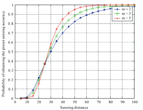
[image:5.595.151.445.527.718.2]Figure 6. The probability of sensing accuracy vs sensing distance considered different fading figures.
up arrangement, with 50 sensor nodes are applied. It is valuable to note that the lifetime is prolonged under the condition which arranged the sensor nodes considering of two lines up arrangement. The probability of sensing ac- curacy vs sensing distance considered under different fading channel is illustrated in Figure 6. The severe situ- ations of fading is quantied with the fading parameters, m
= 2, 3, 5, in this simulation. It is easy to observe that the accuracy will become outperform when the values of fading parameter promoted. Especially, the phenomenon is more significant when the sensing distance is far away the fusion center.
5. Conclusion
The issue of lifetim . The m
REFERENCES
2.15 WPAN™ Task Group 4 (TG4), http://www.ieee802.org/15/pub/TG4.html
[2] X. Wang, et al., “On Data Fusion and Lifetime Constrains in Wireless Sensor Networks,” Proceeding of IEEE In-ternational Conference on Communications, Glasgow, 24-28 June 2007, pp. 3942-3947.
[3] W. R. Heinzelman, A. Chandrakasan and H. Balakrish- man, “An Application-Specific Protocol Architecture for Wireless Micro Sensor Network,” IEEE Transaction on Wireless Communications, Vol. 1, No. 4, 2002, pp. 660- 670. doi:10.1109/TWC.2002.804190
[4] X. D. Wang, et al., “On Data Fusion and Lifetime Con- straints in Wireless Sensor Network,” Proceeding ofIEEE International Conference on Communications, Glasgow, 24-28 June 2007, pp. 3942-3947,.
[5] J.-F. Chamberland and V. V. Veeravalli, “Asymptoic Re- sults for Decentralized Detection in Power Constrained Wireless Sensor Networks,” IEEE Journal on Selected pp. 1007-
e performance is analyzed in this pa- ain reasons to promote the energy efficient, per
increase sensing accuracy and prolong the lifetime of sensor nodes for WSNs (wireless sensor networks) is described. On the basis of adopting sensor management includes sensor movements sequence and sensor location arrangement, we address the issue of lifetime require- ment for sensor nodes which deployed in a surveillance nodes and the data fusion center. The numerical results which definitely show that different arrangement meth- ods are not only able to improve the energy efficient suf- ficiently, but the sensing accuracy and the lifetime of the sensor nodes are also obtained significantly promoted.
[1] IEEE, IEEE 80
Areas in Communications, Vol. 22, No. 6, 2004, 1015. doi:10.1109/JSAC.2004.830894
[6] J. Li and G. AlRegib, “Function-Based Network Lifetime for Estimation in Wireless Sensor Networks,” IEEE Sig-nal Processing Letters, Vol. 15, 2008, pp. 533-536. doi:10.1109/LSP.2008.926499
[7] S. Basagni, A. Carosi, E. Melachrinoudis, C. Petrioli and Z. M. Wang “Controlled Sink Mobility for Prolonging Wireless Sensor Networks Lifetime,” Wireless Networks, Vol. 14, No. 6, 2008, pp. 831-858.
doi:10.1007/s11276-007-0017-x
[8] Y. Y. Yang, M. I. Fonoage and M. Cardei “Improving Net- work Lifetime with Mobile Wireless Sensor Networks,” Computer Communications, Vol. 33, No. 4, 2010, pp. 409- 419. doi:10.1016/j.comcom.2009.11.010
[10] M. Marta and nk Mobility to
In-crease Wirele fetime,” World of
os Angeles, 11-13 Apri
ce on Advanced
In-3-577.
ribution—A General Formula M. Cardei, “Using Si
ss Sensor Networks Li
for
Wireless, Mobile and Multimedia Networks, Newport Be 23-26 June 2008, pp. 1-10.
ach, [13] S. Maheswararajah and S. Halgamuge, “Sensor Schedul- ing for Target Tracking Using Particle Swarm Optimiza- tion,” IEEE 63rdVehicular Technology Conference,Vol. 2, Melbourne, 7-10 May 2006, pp. 57
[11] Y. Z. Bi, J. W. Niu, L. M. Sun, H. F. Wei and Y. Sun, “Moving Schemes for Mobile Sinks in Wireless Sensor Networks,” IEEE International Performance, Computing, and Communications Conference, L l
[1
2007, pp. 101-108.
[12] T. Yang, M. Ikeda, G. Mino, L. Barolli, A. Durresi and F. Xhafa, “Performance Evaluation of Wireless Sensor Net- works for Mobile Sink Considering Consumed Energy Metric,” IEEE International Conferen
of In
mation Networking and Applications Workshops, Perth, 20-23 April 2010, pp. 245-250.
4] T. S. Rappaport, “Wireless Communication, Principles and Practice,” 2nd Edition, Prentice Hall Inc., Upper Sad-dle River, 2002.
[15] M. Nakagami, “The m-Dist