Decoupling Sparsity and Smoothness in the Dirichlet
Variational Autoencoder Topic Model
Sophie Burkhardt [email protected]
Stefan Kramer [email protected]
University of Mainz
Department of Computer Science Staudingerweg 9
55128 Mainz, Germany
Editor:Mohammad Emtiyaz Khan
Abstract
Recent work on variational autoencoders (VAEs) has enabled the development of generative topic models using neural networks. Topic models based on latent Dirichlet allocation (LDA) successfully use the Dirichlet distribution as a prior for the topic and word distributions to enforce sparseness. However, there is a trade-off between sparsity and smoothness in Dirichlet distributions. Sparsity is important for a low reconstruction error during training of the autoencoder, whereas smoothness enables generalization and leads to a better log-likelihood of the test data. Both of these properties are encoded in the Dirichlet parameter vector. By rewriting this parameter vector into a product of a sparse binary vector and a smoothness vector, we decouple the two properties, leading to a model that features both a competitive topic coherence and a high log-likelihood. Efficient training is enabled using rejection sampling variational inference for the reparameterization of the Dirichlet distribution. Our experiments show that our method is competitive with other recent VAE topic models.
Keywords: variational autoencoders, topic models, Dirichlet distribution, reparameteri-zation, generative models
1. Introduction
Generative models have been successfully employed for the modeling of text data since they allow to learn a model of the data and thus are highly interpretable. The arguably most successful model of this kind has been latent Dirichlet allocation (LDA, Blei et al., 2003), which represents each document as a mixture of different topics. This model is typically trained using either Markov chain Monte Carlo (Griffiths and Steyvers, 2004) or variational Bayes (Blei et al., 2003). Recently, several approaches were put forward to train LDA using variational autoencoder neural networks (Miao et al., 2016; Srivastava and Sutton, 2017), thus making them more easily adaptable and extendable by using advances from deep learning research.
Using a Dirichlet distribution as a prior for the latent variables has advantages and disadvantages. The biggest advantage is the sparsity that it encourages in the latent variables. However, we find that the desired sparsity is at odds with the generalization performance of the model. This was previously noticed by Wang and Blei (2009) who
c
tried to decouple sparsity and smoothness in the discrete hierarchical Dirichlet process. In the case of variational autoencoders (VAEs), the problem can be analyzed in terms of the KL-divergence between two Dirichlet distributions, which diverges if the prior parameter is close to zero. Therefore, we are faced with a trade-off: Either the model is sparse and achieves a good reconstruction error, but has a high KL-divergence term and thus a low log-likelihood of the model, or, it avoids low settings of the prior and thereby achieves a better log-likelihood at the cost of a higher reconstruction error. A similar observation was made by Srivastava and Sutton (2018) who observe that a slow minimization of the KL-divergence leads to better topics. In this paper we will discuss how this trade-off can be avoided to achieve both sparsity and smoothness in a variational autoencoder Dirichlet topic model.
One remaining problem with the training of generative models using variational autoen-coders is the need for a differentiable non-centered reparameterization function (Kingma and Welling, 2014a) for the distribution of the latent variables. Unfortunately such a function is not available for the most widely used probability distribution in topic modeling, the Dirichlet distribution. A model that does not directly reparameterize the Dirichlet distribution is ProdLDA (Srivastava and Sutton, 2017) which employs a Laplace approximation for the Dirichlet distribution, thus enabling the training of a Dirichlet variational autoencoder. Other recent solutions include implicit reparameterization gradients (Figurnov et al., 2018), using an approximation for the inverse CDF (Joo et al., 2019) and using the Weibull distri-bution as a replacement (Zhang et al., 2018). In this work we will instead apply rejection sampling variational inference (Naesseth et al., 2017) to autoencoders.
The contributions of our paper are as follows:
1. We introduce a Dirichlet variational autoencoder based on RSVI (DVAE, see
Fig-ure 1a), which is as powerful and efficient as the Gaussian variational autoencoders except it uses the Dirichlet distribution as a prior on the latent variables.
2. We identify the trade-off between sparsity and smoothness as the main factor that prevents successful training of DVAEtopic models and identify the KL-divergence
between two Dirichlet distributions as the crucial factor influencing model performance.
3. We provide an adapted neural network architecture to decouple sparsity and smooth-ness.
4. We show that our Dirichlet variational autoencoder has an improved topic coher-ence, whereas the adapted sparse Dirichlet variational autoencoder has a competitive perplexity.
5. We propose to use the new topic redundancy measure to obtain further information on topic quality when topic coherence scores are high.
2. Related Work
Variational autoencoders (VAEs) were first introduced by Kingma and Welling (2014b) and Rezende et al. (2014). These type of deep neural networks combine ideas from approximate Bayesian inference and deep neural networks, yielding generative models that can be trained by neural networks. Models are trained by stochastic backpropagation using the reparameterization trick. This trick allows the gradient to be backpropagated through the stochastic latent variables efficiently if a reparameterization is available as is the case for the Gaussian distribution.
Topic models based on latent Dirichlet allocation (LDA) (Blei et al., 2003) are directed generative models, which makes it possible to train such topic models using variational autoencoders. The first such neural variational document model (NVDM) was developed by Miao et al. (2016). This model successfully uses the idea of variational autoencoders to train a topic model with a Gaussian prior for the latent variables. This work was extended by Miao et al. (2017), who introduce Gaussian stick breaking priors in a model which is able to let the number of topics grow dynamically.
Another model using Dirichlet stick-breaking priors is SB-VAE (Nalisnick and Smyth, 2017), however, it requires Taylor expansion to compute the KL-divergence and a Ku-maraswamy distribution to approximate the posterior. Since it uses a nonparametric stick-breaking prior instead of a parametric Dirichlet it is not directly comparable to our model.
LDA topic models use a Dirichlet distribution as a prior for the latent variables since it promotes sparsity and leads to more interpretable topics. Therefore, Srivastava and Sutton (2017) propose a VAE topic model called ProdLDA that employs a Laplace approximation for modeling a Dirichlet prior of the latent variables. As their results show, while the perplexity is not as good as that of previous models, the topic coherence is significantly improved over Gaussian VAEs. They also show that the Dirichlet prior leads to more sparseness in the document-topic distributions. This work is extended by Srivastava and Sutton (2018) who introduce a hierarchical VAE topic model. Their analysis shows that batch normalization leads to a slower minimization of the KL-divergence which improves the topic quality.
The reason that VAEs cannot be directly trained using a Dirichlet prior is that there is no simple variable transformation for the Dirichlet distribution. Whereas a Gaussian variable
z∼N(µ, σ2) can be reparameterized asz=µ+σ, ∼N(0,1) thus allowing the gradient to be backpropagated through the latent variablez, there is no such reparameterization for the Dirichlet distribution. However, there is a method to solve this problem which is based on rejection samplers (Naesseth et al., 2017), called RSVI. The Dirichlet distribution can be represented by gamma distributions for which there exists an efficient rejection sampler. The proposal function of this rejection sampler can be used for reparameterization with one minor difference: A correction term has to be added to the gradient that accounts for the difference between the proposal function and the true gamma distribution. In this paper we show how this elegant method can be used for efficient and effective training of Dirichlet variational autoencoders.
distribution is reparameterizable. Zhang et al. (2018) also compare their model with a model trained using RSVI. Overall, their model structure is different however, with a hierarchical generative distribution and a hybrid training algorithm.
Other recent solutions include implicit reparameterization gradients by Figurnov et al. (2018) who introduce a trick to avoid inverting the CDF by differentiating it instead. Furthermore, Joo et al. (2019) use an approximation for the inverse CDF of the gamma distribution. We compare to both of these methods (see Section 5.3 for details).
Our work draws significant inspiration from Wang and Blei (2009). This work is concerned with the HDP-LDA topic model which corresponds to a hierarchical Dirichlet process (HDP) applied to text, resulting in the nonparametric version of latent Dirichlet allocation (Blei et al., 2003). The model represents topics by multinomial distributions over words β ∼Dir(γ), whereβ is the parameter vector of the multinomial distribution which is drawn from a Dirichlet distribution with parameterγ. The decoupling of sparsity and smoothness is applied to these probability distributions β, such that first the words are identified that contribute to the topic and then the Dirichlet distribution is only over the sparse word vector, i.e. a reduced probability simplex. The sparsity is modeled by assuming the topics are generated asβ ∼Dir(b·γ), whereb is a vector of Bernoulli variables with a Beta prior. In contrast, we apply the decoupling to the document-topic distributions instead of the word-topic distributions.
3. Background
In this section, we first introduce LDA topic models. We then explain how topic models are trained with variational autoencoders and how the variational autoencoders can be adapted to use the Dirichlet distribution as a prior for the latent variables.
3.1. LDA
Please note that the notation in this subsection follows the established conventions in topic modeling work. The rest of the paper may use the same variable names in different contexts.
Topic models based on latent Dirichlet allocation (LDA) describe each document in a collection of text documents as a mixture of topics. This means that each document dis associated with a document-topic distributionθd∼Dir(α) with a Dirichlet prior. For each wordwi, a topicziis drawn fromθdand the wordwi is drawn from a topic-word distribution
φzi associated with the topic zi. The joint distribution of the latent variables z, θ andφ is then optimized to maximize the marginal log-likelihood of the dataD under the given model,
L(D|θ, φ, z) = X d∈D
logp(d|z, θ, φ). (1)
3.2. Variational Autoencoders
on VAEs, we adopt the notation common to VAEs here, although it is exactly reversed compared to the topic model notation.
Following Kingma and Welling (2014b), we define a generative model with a latent variable
z and an observed inputx that are generated from a generative distribution pθ(z)pθ(x|z) with parameters θ. This generative model corresponds to the reconstruction/decoder part of the VAE, whereas the encoder corresponds to the variational approximation qφ(z|x) parameterized byφ.
VAEs are generative models similar to LDA topic models. Accordingly, the input data x
is assumed to be generated from a conditional distribution pθ(x|z). The latent topic vectors
z are generated from a prior distributionpθ(z). Generally, it is assumed that the integral of the marginal likelihood pθ(x) =
R
pθ(z)pθ(x|z)dz is intractable as well as the posterior and the integrals required for mean-field variational Bayes. In the case of LDA, it is possible to train the model using mean-field variational Bayes, however, this restricts the model and does not easily allow for certain modifications. For example, using VAEs, it is easily possible to lift the restriction of the mixture model by removing the constraint on the parameters θ, which makes the model more expressive (Srivastava and Sutton, 2017).
The marginal log-likelihood of the model is given by
logp(x) = N
X
i=1
logp(xi) = N
X
i=1
(KL[q(zi|xi)kp(zi|xi)] +L(θ, φ;xi)),
where N is the number of documents in the data set.
Since the KL-divergence is always positive, the second term is the variational lower boundL, which can be written as
logp(xi)≥ L(θ, φ;xi) =Eq(z|xi)[−logq(z|xi)] +Eq(z|xi)[logp(xi, z)] = −KL[q(zi|xi)kp(zi)] +Eq(zi|xi)[logp(xi|zi)],
where the first term in the second line corresponds to the entropy and the second term in the last line corresponds to the negative reconstruction error, whereas the KL-divergence acts as a regularizer that keeps the variational distribution close to the prior. To form an estimate of the ELBO, we need to samplez fromqφand calculate the ELBO by accumulating the contributions of the samples
˜
L(θ, φ;xi) = 1
L
L
X
l=1
(logp(xi, zi,l)−logq(zi,l|xi)),
where Ldenotes the number of samples.
3.3. Rejection Sampling Variational Inference
The Dirichlet distribution can be simulated using gamma random variables since if
zi ∼Γ(αi) then ˜z1:K = Pz1:K
izi ∼Dirichlet(α1:K). This is relevant because for the gamma distribution there exists an efficient rejection sampler
z=hΓ(, α) := (α− 1 3)(1 +
√
9α−3)
3, ∼N(0,1). (2) However, using this proposal function is not equivalent to using a gamma distribution because some samples are rejected. Therefore we need the distribution of an accepted sample
∼s(), which is obtained by marginalizing over the uniform variable u of the rejection sampler,
π(;θ) =
Z
π(, u;θ)du=s() q(h(, θ))
Mθr(h(, θ))
,
where r is the proposal function for the rejection sampler, z = h(, θ), ∼ s() is the reparameterization of the proposal distribution andMθ is a constant used in the rejection sampler. Using this, the ELBO can be rewritten as
Eq(z|xi)[−logq(z|xi)] +Eq(z|xi)[logp(xi, z)] =
Eq(z|xi)[−logq(z|xi)] +Eπ(;θ)[logp(xi, h(, θ))]
As Naesseth et al. (2017) show, the gradient can then be decomposed into three parts
∇θL(θ) =grep +gcor +∇θEq(z|xi)[−logq(z|xi)], (3) where grep andgcor for the case of a one-sample Monte Carlo estimator are given as
grep =∇zlogp(xi, z)∇θh(, θ),
gcor = logp(xi, z)∇θlog
q(h(, θ))
r(h(, θ)),
and the entropy can be calculated analytically. grep corresponds to the gradient assuming
that the proposal is exact and always accepted andgcor corresponds to a correction part of the gradient that accounts for not using an exact proposal.
3.4. Shape Augmentation for Gamma Distribution
The rejection sampler for the gamma distribution has higher acceptance rates for higher values of the parameterα. Naesseth et al. (2017) use this fact to augment the shape of the gamma distribution and thereby achieve a lower variance gradient. As they show, a Γ(α,1)
distributed variablez can be expressed as z= ˜zQB
i=1u
1
α+i−1
i for a positive integerB and i.i.d. uniform random variables u, where ˜z∼Γ(α+B,1). This makes it possible to use the rejection sampler forα <1 and also decreases the correction term for increasing α+B.
4. Method
4.1. Sparsity and Smoothness
The trade-off between sparsity and smoothness is a known issue in the topic modeling literature (Wang and Blei, 2009). Aspects of it were also discussed in recent literature by Srivastava and Sutton (2017, 2018). According to them, batch normalization and dropout slow down the minimization of the KL-divergence in the beginning of training. This has the effect of increasing the smoothness and thereby increases the topic coherence because the model generalizes better. A fast minimization puts a greater emphasis on sparseness which ensures a lower perplexity, but is prone to overfitting. A minimization that is too fast leads to maximal smoothness which means the Dirichlet parameter is equal to the prior. In this case no meaningful topics can be learned since the latent variables are only sampling noise. This problem is known as component collapsing.
But influencing the training process through e.g. batch normalization or dropout is only one way to control this trade-off. By decoupling both aspects explicitly we can allow both, a good generalization performance and a good fit to the data at hand. To do this, first, the topics are selected that represent the current document. Second, a distribution is sampled for the selected topics. The details are described in the next section.
4.2. DVAE Sparse
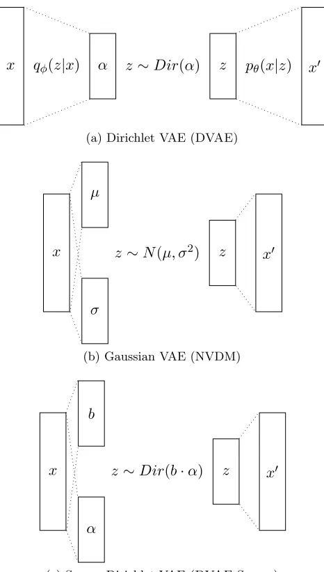
A schematic view of our methods is depicted in Figures 1a and 1c. We will now describe the sparse Dirichlet variational autoencoder (DVAESparse) depicted in Figure 1c. The DVAE
model works analogously except that the vector bis set to a vector of only ones. The model equation is given byp(x, z, θ) =p(x|z, θ)·p(z|θ)·p(θ). The inputx is transformed to the Dirichlet parameter αand a sparsity parameter bby a neural network, the latent variablesz
are sampled from Dir(b·α) and the decoder network reconstructs the original input. This is in contrast to the Gaussian autoencoder shown in Figure 1b, where the latent variables are drawn from a Gaussian distribution. To be able to backpropagate the gradients through the latent variables z, we use rejection sampling variational inference.
The parameter b is inspired by Wang and Blei (2009), who use a Bernoulli distributed variable. In contrast, we simply use a sigmoid function and subsequently round the result to zero or one. The distribution Dir(b·α) is a degenerate Dirichlet distribution over the sub-simplex specified by
b=l2(λ) = round( 1 1 +e−λ).
If the vectorbonly consists of ones, this reduces to the normal Dirichlet distributionDir(α). We optimize α in an unconstrained domain by letting
α= log(1 + exp(a)), (4)
where a =l1(λ) is a linear transformation of λ and λis the transformation of the input through the neural networkλ=fMLP(x).
The ELBO is given by
x qφ(z|x) α z∼Dir(α) z pθ(x|z) x0
(a) Dirichlet VAE (DVAE)
x µ
σ
z∼N(µ, σ2) z x0
(b) Gaussian VAE (NVDM)
x b
α
z∼Dir(b·α) z x0
(c) Sparse Dirichlet VAE (DVAESparse)
Figure 1: Schematic figure of Dirichlet VAE, Gaussian VAE and the proposed Sparse Dirichlet VAE. For the Dirichlet VAE the input is transformed by a neural network to yield parameter α. The latent variables z are subsequently sampled fromDir(α). Finally the input is reconstructed asx0. The Gaussian VAE has parametersµand
σ instead and uses a Gaussian distribution.
Here, the expectation representing the negative reconstruction error is rephrased with respect to the distribution of the accepted sampleπand the latent variableszare reparameterized by
hΓ(, φ) given in Equation 2. π(;φ), the distribution of the accepted sample, is obtained by marginalizing over the uniform variable u,
π(;φ) =
Z
π(, u;φ)du=s()q(hΓ(, φ))
r(hΓ(, φ))
x
λ=RELU(linear(x))
λ=Dropout(λ)
λ
l1=linear(λ)
l1
l1=Batchnorm(l1)
α=M ax(0.00001, sof tplus(l1))
α
z∼Dirichlet(α)
z
l2 =linear(z)
l2
l2=Batchnorm(l2)
x0 =Log Sof tmax(l2)
x0
Figure 2: Illustration of the neural network architecture used for DVAE, ProdLDA, the
Here, we use the parameterφsince our encoder network is parameterized by φ. The gradient of the ELBO for the generative/decoder network is given as follows:
∇θL(θ, φ;xi) =∇θEq(z|xi)[logp(xi|z)].
This corresponds to the logarithm of the reconstruction probability. Gradient backpropaga-tion for this term is unproblematic since the samples used to estimateL depend onq which is parameterized by φ. Therefore we do not need to take care of reparameterization for this term. The gradients of the ELBO for the the variational/encoder network are as follows:
∇φL(θ, φ;xi) =∇φ−KL[q(z|xi)kp(z)] +∇φEπ(;θ)[logp(xi|hΓ(, φ))] (7) Here, we need to reparameterize the latent variables z. The gradient of the KL-divergence will be discussed in Section 4.3 and the rest of the gradient is given analogously to Equation 3. Note that we now use the expectation of the conditional distribution p(xi|z) instead of the joint distributionp(xi, z), since we write the ELBO in a different way which is more common for VAEs. The gradient based on a one-sample Monte Carlo estimator is given as
∇φL(θ, φ;xi) =∇φ−KL[q(z|xi)kp(z)] +grep +φ gcorφ . (8)
gφrep =∇zlogp(xi|z)∇φh(, φ)
gcor = logφ p(xi|z)∇φlog
q(h(, φ))
r(h(, φ))
To understand the step from Equation 7 to Equation 8, we refer to the derivation by Naesseth et al. (2017),
Eπ(;θ)[f(h(, φ))] =
Z
s()∇φ
f(h(, φ))q(h(, φ);φ)
r(h(, φ);φ)
d=
Z
s()q(h(, φ);φ)
r(h(, φ);φ)∇φf(h(, φ))d+
Z
s()f(h(, φ))∇φ
q(h(, φ);φ)
r(h(, φ);φ)
d=
Eπ(;θ)[∇φf(h(, φ))] +Eπ(;θ)
f(h(, φ))∇φlogq(h(, φ);φ)
r(h(, φ);φ)
,
(9)
where in the last step the log-derivative trick was used andf(h(, φ)) in our case corresponds to logp(xi|h(, φ)).
4.3. The KL-Divergence
The KL-divergence can be calculated analytically, meaning that we do not have to use any samples and thus do not need to take care of reparameterization in the gradient back propagation for this term. p(z) is a Dirichlet with priorα0, whereasq(z|x) is the Dirichlet parameterized byα as given by the variational network parameterized by φ.
KL[q(z|x)kp(z)] = log(Γ(X k
αk))−log(Γ(
X
k
α0k))+
X
k
log Γ(α0k)−X k
log Γ(αk) +
X
k
(αk−α0k)(Ψ(α)−Ψ(
X
k
where Ψ is the digamma function.
In our experiments we found that the analytical calculation of the KL-divergence, even though it is theoretically more appealing, does not lead to optimal results. We therefore resort to using a simple sampling approximation of the KL-divergence by calculating the KL-divergence as KL[q(z|x)kp(z)] =q(z|x) logqp(z(z|x)). Note that test results are calculated using the analytical KL-divergence to enable a fair comparison. Sampling the KL-divergence leads to more stable gradients, however, it introduces a second correction term for the gradient of the encoder network, since we are now using the rejection sampler again to producez.
We therefore rewrite the ELBO as
L(θ, φ;xi) =−KL[q(z|xi)kp(z)] +Eq(z|xi)[logp(xi|z)] =
Eπ(;φ)
log p(hΓ(, φ))
q(hΓ(, φ)|x)
+Eπ(;φ)[logp(xi|hΓ(, φ))]. The gradient of the KL-divergence is now given as
∇φKL[q(hΓ(, φ))|x)kp(hΓ(, φ))] =∇φlog
p(hΓ(, φ))
q(hΓ(, φ)|x) +gφ
kl-cor, (10)
where gφ
kl-coris defined as
gφ
kl-cor= log
p(hΓ(, φ))
q(hΓ(, φ)|x)∇φlog
q(hΓ(, φ))
r(hΓ(, φ)).
The log fraction in this correction term is the same as the one for gcor, however, it isφ
weighted by the KL-divergence instead of the reconstruction probability. The derivation is again done using Equation 9 except nowf(h(, φ)) corresponds to logq(hp(,φ(z))|x). Note, that the two terms in Equation 10 correspond to a reparameterization part and a score function part. If the proposal is equal to the distribution and always accepted this reduces to the reparameterization gradient, whereas if the proposal is always rejected, this reduces to the score function gradient, also known as REINFORCE.1
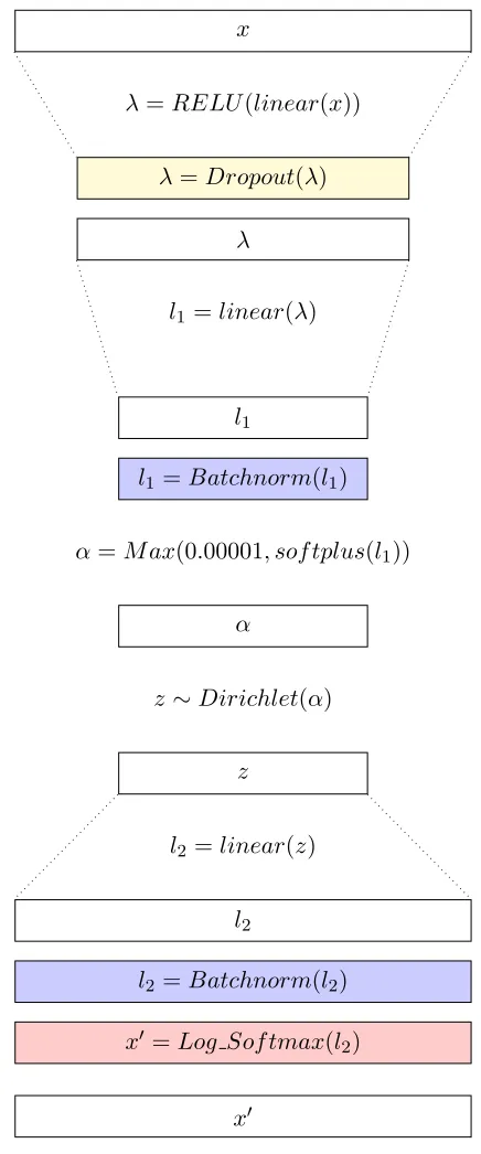
4.4. Neural Network Architecture
The architecture of the neural network for the DVAEvariational autoencoder is illustrated
in Figure 2.
1. Encoder: The input is transformed using a RELU-layer with dropout. The result is linearly transformed and batch normalization is applied. Batch normalization is crucial for the convergence of the model. VAEs are prone to so-called component collapsing, a well-known problem (Bowman et al., 2016). Using batch normalization in combination with a relatively high learning rate (10−2–10−4), helps to avoid component collapsing and leads to a fast convergence (Srivastava and Sutton, 2017). A softplus transformation is applied because the Dirichlet parameter needs to be positive. Furthermore, a
minimum value of 0.00001 is used for the Dirichlet parameter α which is necessary for stability of the gradients. The latent variables z are sampled from the Dirichlet distribution.
2. Decoder: The decoder is structured as follows: The latent variables zare transformed linearly. Again, batch normalization is applied. The final result is obtained through a log-softmax transformation. Note that the decoder weights are not restricted to be on the probability simplex as would be necessary if a Dirichlet prior was put on the topic-word distributions. This lifts the restriction of the mixture model as proposed by Srivastava and Sutton (2017) (The same was done in the NVDM model by Miao et al. (2016), although it was not explicitly discussed.). This is why in our experiments we
compare to the ProdLDA model of Srivastava and Sutton (2017) and not to AVITM, which puts the simplex constraint on the decoder weights. Nevertheless, we can use the decoder weights to infer our topics since it is sufficient to rank the words according to the respective weights for each topic. The weights do not have be given a probabilistic interpretation as in LDA models. The words with the largest weights for each latent topic, are usually representative for that topic. It was shown by Srivastava and Sutton (2017) and is confirmed in our experiments that the non-mixture version yields lower perplexity but higher topic coherence. The reason for this is suspected to be the lifting of the mixture model contraint which makes the model more expressive.
4.5. Component Collapsing
As mentioned in the previous section, VAEs often suffer from the well-known issue of component collapsing (Bowman et al., 2016). This is the problem of a local minimum that is usually encountered early on in the training process and which the model cannot escape as the training continues. It occurs because it is often easier for the model to minimize the KL-divergence than to minimize the reconstruction error. This leads to parameters that are equal to the prior and thus, many or all topics are the same. This means that there are a lot of redundant topics, but the perplexity is relatively low. To prevent this from happening, a common method is annealing of the KL-divergence (Bowman et al., 2016) to slowly introduce it into the loss function. Other methods include batch normalization and dropout (Srivastava and Sutton, 2017, 2018). In our experiments, we found that batch normalization had the largest effect. None of the implemented Dirichlet autoencoders learn meaningful topics without batch normalization. NVDM does not employ batch normalization, but has to use a lower learning rate to prevent component collapsing.
5. Experiments
Here, we first describe the experimental settings, the data sets, baseline methods and the evaluation measures. Finally we describe the experimental results on the different performance measures.
5.1. Experimental Settings
models. Training was monitored on a validation set with early stopping and a look-ahead of 30 iterations. We used the Adam optimizer for training. For NVDM each training iteration spans ten iterations for the decoder and ten iterations for the encoder. DVAEand ProdLDA
optimize decoder and encoder jointly. Since we noticed that DVAE has no difference in
performance between using the correction part of the gradient when shape augmentation is used, we omitted that part in the experiments to save unnecessary computation. Similar to Srivastava and Sutton (2017), we employ batch normalization to improve the convergence of our model. The learning rate is optimized for all neural network methods using Bayesian optimization.
5.2. Data Sets
• 20news: We used the same version of this data set as Srivastava and Sutton (2017). It is a widely used text data set consisting of news articles that are grouped into 20 different categories. It has 11,000 training instances and a 2,000 word vocabulary.
• NIPS: The NIPS data set was retrieved in a preprocessed format from the UCI Machine Learning Repository (Perrone et al., 2017). It consist of 5,812 documents and has 11,463 features. It contains text data from NIPS conference papers published between 1987 and 2015. Compared to the other data sets, individual documents are large. 1,000 documents were separated as a test set.
• KOS: The 3,430 blog entries of this data set were originally extracted from http: //www.dailykos.com/, the data set is available in the UCI Machine Learning Repos-itoryhttps://archive.ics.uci.edu/ml/datasets/Bag+of+Words. The number of features is 6,906.
• Rcv1:2 This corpus contains 810,000 documents of Reuters news stories. We separated 10,000 documents as a testset and pruned the vocabulary to 10,000 words after stopword removal following Miao et al. (2016).
5.3. Methods
5.3.1. Dirichlet Autoencoders
We compare to four different autoencoders that all have exactly the same architecture and hyperparameters as DVAE. They are only different with respect to the modeling of the
Dirichlet prior on the latent variables.
1. ProdLDA: This method uses a Laplace approximation to approximate the Dirichlet prior. We use the implementation provided by the authors.3
2. Inverse CDF (Joo et al., 2019): This method builds on previous work by Knowles (2015). IfX ∼Γ(α, β) andF(x;α, β) is a CDF of the random variableX, the inverse CDF can be approximated by F−1(u;α, β) ≈β−1(uαΓ(α))1/α, where u ∼Uniform(0,1). The approximated inverse CDF can then be used as a reparameterization function.
2.http://trec.nist.gov/data/reuters/reuters.html
3. Implicit reparameterization gradients (Figurnov et al., 2018): This method introduces a trick to avoid inverting the CDF by differentiating it instead. It is integrated into the tensorflow library and can be used out-of-the-box.
4. Weibull autoencoder (Zhang et al., 2018): This method uses the Weibull distribution instead of the Gamma distribution because it has a similar PDF and the Weibull distribution can be reparameterized easily. The Weibull PDF is given as
P(x|k, λweibull) = k λk
weibull
xk−1exp (x/λweibull)k.
The reparameterization for x∼W eibull(k, λweibull) is
x=λ(−ln(1−))1/k, ∼Uniform(0,1),
and the KL-divergence from the gamma distribution is analytically computed as
KL[W eibull(k, λweibull)kGamma(α, β)] =
αlnλweibull−γα
k −lnk−βλweibullΓ
1 +1
k
+γ+ 1 +αlnβ−ln Γ(α).
The parameters λweibull and kare computed through the neural network as
λweibull = log(1 + exp(b)), k= log(1 + exp(c)),
where b=l2(λ) and c=l3(λ), where l2 and l3 are linear transformations ofλwhich is the same as in Equation 4.
Additionally, k is restricted to be greater or equal to 0.1 because for values of kthat are lower than that the method becomes unstable.
5.3.2. Other Comparison Methods
Additionally, we compare to two other algorithms:
1. NVDM: This is the Gaussian VAE topic model. We used the code provided by the authors.4
2. SCVB: As a representative of the original LDA models, we compare to SCVB (Foulds et al., 2013), a stochastic variant of collapsed variational Bayes. This method is trained online using minibatches in the same way as the neural networks. Therefore the method is applicable to large data sets. We used our own Java reimplementation.
5.4. Evaluation
All models are evaluated on three measures, perplexity, topic redundancy and topic coherence. The per-word perplexity is calculated from the ELBO as exp(− 1
Nw
PD
d logp(d)), where Nw is the number of words in the corpus. We use the analytical KL-divergence for all models to calculate the perplexity to allow a fair comparison.
The topic coherence is calculated following Srivastava and Sutton (2017) using the normalized pointwise mutual information (NPMI), averaged over all pairs of words of all topics, where the NPMI is set to zero for the case that a word pair does not occur together. We calculate the topic coherence on the test set using the 10 first words of each topic, i.e. the 10 words with the highest probability for that topic. The NPMI for topict is given as follows:
NPMI(t) = N X
j=2 j−1
X
i=1
log P(wj,wi) P(wi)P(wj) −logP(wi, wj)
,
where N is the number of words in topict, wi is theith word of topictandP(wi, wj) is the probability of wordswi and wj occurring together in the test set, which is approximated by counting the number of documents where both words appear together5 and dividing the result by the total number of documents.
The topic redundancy corresponds to the average probability of each word to occur in one of the other topics of the same model. The redundancy for topick is thus given as
R(k) = 1
K−1 N
X
i=1
X
j6=k
P(wik, j),
where P(wik, j) is one if the ith word of topic k,wik, occurs in topicj and otherwise zero, and K−1 is the number of topics excluding the current topic.
5.5. Experimental Results
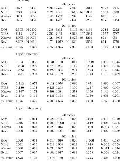
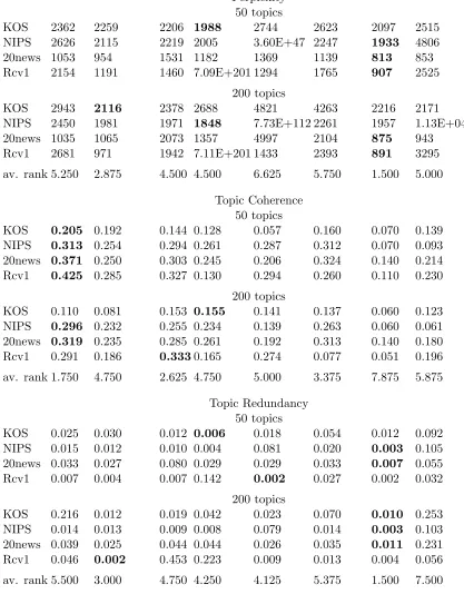
5.5.1. Perplexity
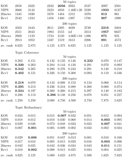
We compare our models,DVAEandDVAESparse, to the Laplace approximationProdLDA,
the Gaussian VAE NVDM and the online LDA model SCVB in Tables 1 and 2. Additional results are in the Appendix in Tables 4 and 5. The overall best perplexity is achieved by NVDM as can be seen from the average ranks in each table, whereas the Weibull VAE has the worst perplexity, closely followed by DVAE. Implicit gradients VAE and inverse
CDF VAE are worse than NVDM and DVAESparse, but a little bit better than DVAE
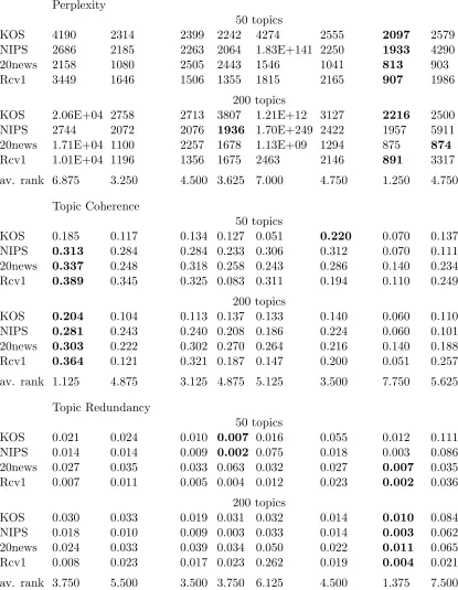
and Weibull VAE. The reason for the high perplexity of DVAE is the KL-divergence part
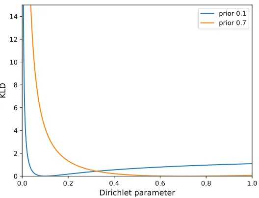
of the ELBO (Equation 6). The KL-divergence between two Dirichlet distributions can have extreme values as shown in Figure 3. If the Dirichlet parameter is close to zero, the KL-divergence and therefore also the perplexity is high. As Tables 1 and 2 show, theDVAE
Sparse model successfully circumvents this problem by decoupling sparsity and smoothness. The perplexity of DVAE Sparse, while not as good as that of NVDM, is mostly better or at
least comparable to that of the ProdLDA model.
data set DVAE DVAESp. Impl. Inv. Weibull ProdLDA NVDM SCVB
Perplexity
50 topics
KOS 7872 2408 2894 2598 7795 2811 2097 2365
NIPS 2779 2197 2327 2141 3.55E+52 2303 1933 3973
20news 5009 1066 1842 1533 5209 1128 813 817
Rcv1 5885 1464 1635 1547 2344 2265 907 2034
200 topics
KOS 2.59E+05 2397 3238 3233 3.11E+04 3161 2216 2222 NIPS 3110 2152 2250 2135 8.50E+167 2532 1957 5787 20news 4.93E+05 1075 3021 3033 1.82E+08 1271 875 951 Rcv1 8.66E+04 1614 1471 1.07E+10 4426 2559 891 2779
av. rank 7.125 2.875 4.750 4.375 7.375 4.500 1.000 4.000
Topic Coherence
50 topics
KOS 0.194 0.050 0.131 0.130 0.067 0.218 0.070 0.145
NIPS 0.313 0.295 0.276 0.224 0.167 0.293 0.070 0.116
20news 0.324 0.248 0.322 0.304 0.271 0.223 0.140 0.244
Rcv1 0.381 0.293 0.340 0.162 0.216 0.140 0.110 0.239
200 topics
KOS 0.212 0.072 0.118 0.076 0.086 0.071 0.060 0.107
NIPS 0.280 0.234 0.227 0.208 0.176 0.277 0.060 0.105
20news 0.307 0.174 0.298 0.281 0.258 0.150 0.140 0.204
Rcv1 0.373 0.115 0.237 0.138 0.069 0.370 0.051 0.263
av. rank 1.125 4.875 3.000 4.625 5.375 4.500 7.750 4.750
Topic Redundancy
50 topics
KOS 0.017 0.014 0.024 0.011 0.020 0.040 0.012 0.110 NIPS 0.016 0.013 0.008 0.003 0.123 0.019 0.003 0.088 20news 0.026 0.025 0.022 0.018 0.039 0.020 0.007 0.037 Rcv1 0.009 0.269 0.002 0.001 0.095 0.017 0.002 0.039
200 topics
KOS 0.026 0.013 0.016 0.010 0.020 0.006 0.010 0.088 NIPS 0.021 0.010 0.012 0.008 0.022 0.018 0.003 0.058 20news 0.030 0.016 0.030 0.027 0.044 0.013 0.011 0.046 Rcv1 0.007 0.017 0.104 0.817 0.668 0.253 0.004 0.024
av. rank 4.875 4.125 4.375 2.750 6.875 4.375 1.625 7.000
data set DVAE DVAESp. Impl. Inv. Weibull ProdLDA NVDM SCVB
Perplexity
50 topics
KOS 4190 2314 2399 2242 4274 2555 2097 2579
NIPS 2686 2185 2263 2064 1.83E+141 2250 1933 4290
20news 2158 1080 2505 2443 1546 1041 813 903
Rcv1 3449 1646 1506 1355 1815 2165 907 1986
200 topics
KOS 2.06E+04 2758 2713 3807 1.21E+12 3127 2216 2500 NIPS 2744 2072 2076 1936 1.70E+249 2422 1957 5911 20news 1.71E+04 1100 2257 1678 1.13E+09 1294 875 874 Rcv1 1.01E+04 1196 1356 1675 2463 2146 891 3317
av. rank 6.875 3.250 4.500 3.625 7.000 4.750 1.250 4.750
Topic Coherence
50 topics
KOS 0.185 0.117 0.134 0.127 0.051 0.220 0.070 0.137
NIPS 0.313 0.284 0.284 0.233 0.306 0.312 0.070 0.111
20news 0.337 0.248 0.318 0.258 0.243 0.286 0.140 0.234
Rcv1 0.389 0.345 0.325 0.083 0.311 0.194 0.110 0.249
200 topics
KOS 0.204 0.104 0.113 0.137 0.133 0.140 0.060 0.110
NIPS 0.281 0.243 0.240 0.208 0.186 0.224 0.060 0.101
20news 0.303 0.222 0.302 0.270 0.264 0.216 0.140 0.188
Rcv1 0.364 0.121 0.321 0.187 0.147 0.200 0.051 0.257
av. rank 1.125 4.875 3.125 4.875 5.125 3.500 7.750 5.625
Topic Redundancy
50 topics
KOS 0.021 0.024 0.010 0.007 0.016 0.055 0.012 0.111 NIPS 0.014 0.014 0.009 0.002 0.075 0.018 0.003 0.086 20news 0.027 0.035 0.033 0.063 0.032 0.027 0.007 0.035 Rcv1 0.007 0.011 0.005 0.004 0.012 0.023 0.002 0.036
200 topics
KOS 0.030 0.033 0.019 0.031 0.032 0.014 0.010 0.084 NIPS 0.018 0.010 0.009 0.003 0.033 0.014 0.003 0.062 20news 0.024 0.033 0.039 0.034 0.050 0.022 0.011 0.065 Rcv1 0.008 0.023 0.017 0.023 0.262 0.019 0.004 0.021
av. rank 3.750 5.500 3.500 3.750 6.125 4.500 1.375 7.500
0.0 0.2 0.4 0.6 0.8 1.0
Dirichlet parameter
0 2 4 6 8 10 12 14
KLD
prior 0.1 prior 0.7
Figure 3: This plot shows the KL-divergence between two Dirichlet distributions with identical parameters, where only one element of one parameter vector is varied between zero and one. All other elements are fixed to 0.1 (blue line) or 0.7 (orange line). We can see that the KL-divergence diverges for small parameter values.
5.5.2. Topic Coherence
In terms of topic coherence (see Tables 1 and 2, middle section, as well as additional results in the Appendix),DVAEhas consistently high values as compared to all other methods with
the best average rank for all settings of the Dirichlet parameter. A slight decrease in the average rank (1.125,1.125,1.250,1.750) can be observed for increasing values of the Dirichlet parameter which indicates thatDVAEis especially good at modeling the sparseness implied by small parameter settings. DVAE Sparse is slightly worse than ProdLDA, but generally
still better than NVDM and SCVB in terms of the average rank in topic coherence. This shows a trade-off between perplexity and topic coherence which can be influenced through the sparseness of the model. WhileDVAE Sparse has a far better perplexity thanDVAE,
its topic coherence is generally worse. While increased sparseness may thus lead to a lower topic coherence, this is not the only indicator for the topic quality (see Section 5.5.3).
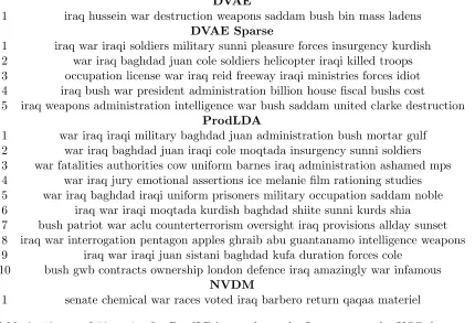
Taking a closer look at the topic outputs, it is not always the case that a higher topic coherence corresponds to better topics. In Table 3 we listed all the topics that ProdLDA learned on the KOS data set that have the words “iraq” and “war” in the most frequent words. This concerns ten out of fifty topics. ProdLDA often learns topics of relatively high quality that are redundant. This way, it is able to achieve a high topic coherence, but the diversity of the topics is not accounted for by this measure. DVAE in contrast learned
only one topic containing the words “iraq” and “war” (see also Table 3), whereasDVAE
0 20 40 60 80 100 #iterations
4000 5000 6000 7000 8000 9000 10000 11000
Perplexity
Perplexity Analytical Training Perplexity Sampled Training
(a) Perplexity
0 20 40 60 80 100
#iterations 85
90 95 100 105 110
KL-Divergence
KLD Analytical Training KLD Sampled Training
(b) KL-divergence
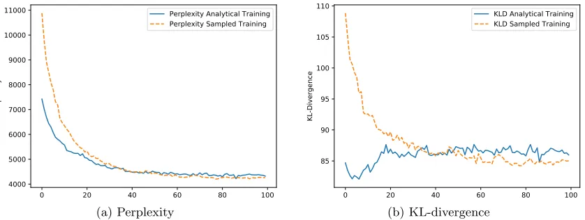
Figure 4: This figure compares the performance of DVAE trained with the analytical
KL-divergence with the performance of DVAE trained with the sampled
KL-divergence on the 20news data set using a Dirichlet prior of 0.02. Reported is the perplexity using the analytical KL-divergence as well as the analytical KL-divergence. We can see that the final perplexity and KL-divergence for the sampled version are lower even though the convergence is slower in the beginning.
single topic on the Iraq war, the quality of this topic is subjectively bad as none of the other words are closely related to the war. Nevertheless, ProdLDA has a topic coherence of 0.22 and DVAEand DVAESparse only reach 0.19 and 0.12, respectively. This shows that,
while topic coherence is considered to be closely related to human judgement about topic quality (Lau et al., 2014), it is not a good indicator of topic quality in the case where topic redundancy is a problem.
Comparing the implicit gradients VAE, inverse CDF VAE and Weibull VAE in term of topic coherence, Tables 1 and 2 show that the implicit gradients method achieves the second best topic coherence overall and is only worse thanDVAE. The inverse CDF and Weibull
methods however, show a topic coherence that is in general comparable to theDVAESparse
method. Judging from the topic coherence results, the approximations that are made by the Weibull and inverse CDF autoencoders are not as good as the implicit gradients and RSVI methods. We can therefore conclude that the RSVI and implicit gradients methods are preferable for Dirichlet parameter settings <1 as are typical in topic modeling. The difference between theDVAE and the implicit gradients VAE method is minimal according
to Figurnov et al. (2018), however, the used Dirichlet parameter is not reported since it was optimized during training. We therefore hypothesize that our improved performance is due to the sampled KL-divergence as well as a better approximation for low settings of the Dirichlet parameter.
5.5.3. Topic Redundancy
DVAE
1 iraq hussein war destruction weapons saddam bush bin mass ladens DVAE Sparse
1 iraq war iraqi soldiers military sunni pleasure forces insurgency kurdish 2 war iraq baghdad juan cole soldiers helicopter iraqi killed troops 3 occupation license war iraq reid freeway iraqi ministries forces idiot 4 iraq bush war president administration billion house fiscal bushs cost
5 iraq weapons administration intelligence war bush saddam united clarke destruction ProdLDA
1 war iraq iraqi military baghdad juan administration bush mortar gulf 2 war iraq baghdad juan iraqi cole moqtada insurgency sunni soldiers 3 war fatalities authorities cow uniform barnes iraq administration ashamed mps 4 war iraq jury emotional assertions ice melanie film rationing studies 5 war iraq baghdad iraqi uniform prisoners military occupation saddam noble 6 iraq war iraqi moqtada kurdish baghdad shiite sunni kurds shia 7 bush patriot war aclu counterterrorism oversight iraq provisions allday sunset 8 iraq war interrogation pentagon apples ghraib abu guantanamo intelligence weapons 9 iraq war iraqi juan sistani baghdad kufa duration forces cole
10 bush gwb contracts ownership london defence iraq amazingly war infamous NVDM
1 senate chemical war races voted iraq barbero return qaqaa materiel
Table 3: 10 out of 50 topics for ProdLDA are about the Iraq war on the KOS data set with a Dirichlet prior of 0.1. The topic coherence is 0.22 for this run, since topic coherence does not account for the diversity of topics. The topic coherence for
DVAESparse is only 0.12, however, the topic quality is higher as can be seen from
the topic redundancy score and qualitatively from this example. For DVAE, only
one topic is about the Iraq war and the topic redundancy score is lower than that of ProdLDA and DVAESparse while the topic coherence is still high.
and 2 show that the lowest redundancy scores were achieved by NVDM, however, NVDM has a far worse topic coherence. In our experience the overall topic quality of all other models was mostly better than that of NVDM. If the topic coherence is low, however, the redundancy score is not that meaningful, since a low redundancy can also be expected from a model that assigns words to topics randomly. If a model achieves a high topic coherence as can be seen in Table 5 for the implicit gradients method with the Rcv1 data set and 200 topics, this can still be associated with a very hight topic redundancy (0.45 in this case) which points to component collapsing and devalues the high topic coherence score. DVAE
6. Discussion
DVAE,DVAE Sparse, implicit gradients VAE, inverse CDF VAE and Weibull VAE are
most closely related to the ProdLDA model. All of these models can be trained with relatively high learning rates (10−3–10−2) as compared to NVDM, which is trained with much lower learning rates (around 10−5). This speeds up the training process considerably. The efficiency of ProdLDA, DVAEand DVAESparse and the other Dirichlet autoencoders
is comparable as long as the correction term is disregarded for theDVAE models. This can
safely be done as long as the shape augmentation parameter is chosen high enough (≥5). The training efficiency might also be affected by other architectural decisions that warrant further investigation in the future. NVDM trains the encoder and decoder networks separately, whereas DVAEand ProdLDA update both networks at once. DVAE and ProdLDA use
dropout and batch normalization, which enable the high learning rates. All these details need to be taken into consideration and their potential influence will be investigated in future work.
All models with a Dirichlet latent parameter vector are characterized by a relatively high topic coherence as compared to the Gaussian model NVDM. This shows that it is worth considering to use the Dirichlet distribution in cases where interpretable topics are important. Nevertheless, topic coherence alone is not a good indicator of topic quality and should be viewed in conjunction with our newly introduced measure of topic redundancy. This is especially important in VAE topic models due to the problem of component collapsing, which is more prevalent in VAEs than in other LDA topic models.
Comparing our two modelsDVAE and DVAE Sparse,DVAE clearly leads to topics of
higher quality. The perplexity, however, is bad in comparison. According to our analysis this is due to the KL-divergence term in the ELBO that leads to high values when the parameter is predicted to be close to zero. By modeling the sparseness in a separate vector, this problem is alleviated, leading to lower perplexities. DVAE Sparse therefore serves as a
test to show that our original hypothesis is correct, namely that the coupling of sparsity and smoothness is responsible for the high perplexity scores. Furthermore, this shows that perplexity scores are not always meaningful when comparing different topic models, as in our experiments the topic quality has nothing to do with the perplexity a model achieves.
the stability problem completely disappear. How such a method could be applied to the variational autoencoder however, remains open.
Our experiments show that DVAEis superior to other state-of-the-art topic models in
terms of topic coherence. This further underlines the argument by Srivastava and Sutton (2017) that the sparsity induced by the Dirichlet indeed leads to higher topic coherence. The comparison with other Dirichlet autoencoders shows that while our version of the RSVI autoencoder works best, the implicit gradients VAE is the most competitive method, whereas the inverse CDF and Weibull autoencoders are even worse than the Laplace approximation of ProdLDA in terms of topic coherence.
We discussed the trade-off between sparsity and smoothness in Section 4.1. This trade-off can be influenced using the DVAE Sparse model with the additional Bernoulli variable.
Furthermore, the sampling of the KL-divergence is an important factor for increasing the topic coherence. As shown in Figure 4, while the convergence of perplexity and KL-divergence seems to be slower in the beginning, this may lead to a lower perplexity and KL-divergence in the final stages of training. For the shown comparison the final topic coherence score was 0.33 for the training method with the analytical KL-divergence, whereas training with the sampled KL-divergence led to a topic coherence of 0.35 after 100 iterations of training. This effect is similar to the effect of batch normalization as reported by Srivastava and Sutton (2018) who did a similar experiment. They show that batch normalization slows down the convergence of the KL-divergence in the beginning of training. This reduces the component collapsing and enables the learning of more meaningful topics.
When talking about a trade-off, this implies that there is a continuum of models between extreme sparseness and extreme smoothness. This can in principle be explored using our
DVAESparse model. While at the moment, the parameter for our Bernoulli variables is p= 0.5, this parameter could also be set to other values and thereby increase or decrease the sparseness of the model. On the one hand, a value of p= 0 would mean that the vector
b will always consist of only ones. This would reduce the model to the original DVAE
model, which is a smooth model. On the other hand, forp= 1 the vectorbwould consist of only zeros, which entails maximal sparseness and only topics with zero values, preventing any topics from being learned. Intermediary values can be used to adjust the degree of sparseness and interpolate between the sparse and the smooth model.
7. Conclusion
We have introduced a variational autoencoder with a Dirichlet prior calledDVAE. A trade-off
between sparsity and smoothness was identified, leading to high perplexity as well as topic coherence scores. To test our hypothesis about the reason for the high perplexity scores, a new model calledDVAE Sparse was introduced. DVAESparse decouples sparsity and
smoothness and thus enables lower perplexity scores on the one hand while on the other hand the topic coherence is still competitive. The topic quality was also measured in terms of topic redundancy which is a good indicator for component collapsing as opposed to topic coherence. Overall, this shows that, despite the bad perplexity scores,DVAE is an effective
To conclude, we think that this work is an important step towards making VAEs with Dirichlet priors more widely used. In the future we would like to extend our model to work with hierarchical Dirichlet priors.
Acknowledgements
We thank the anonymous reviewers for their helpful comments.
data set DVAE DVAE Sp. Impl. Inv. Weibull ProdLDA NVDM SCVB
Perplexity
50 topics
KOS 2858 2322 2232 2056 2923 2537 2097 2501
NIPS 2666 2142 2223 4858 1.46E+26 2239 1933 8137
20news 1345 1030 1678 1484 1212 1076 813 961
Rcv1 2542 1234 1458 1480 1397 1788 907 1990
200 topics
KOS 4503 2443 2611 2395 4839 3739 2216 2404
NIPS 2551 2043 1983 2155 inf 2313 1957 6627
20news 2869 1123 1734 2120 4.66E+04 1496 875 925
Rcv1 2913 1052 1337 1519 1613 2206 891 4573
av. rank 6.625 2.875 4.125 4.375 6.625 5.125 1.125 5.125
Topic Coherence
50 topics
KOS 0.202 0.151 0.132 0.135 0.146 0.232 0.070 0.147
NIPS 0.330 0.263 0.284 0.144 0.120 0.281 0.070 0.093
20news 0.342 0.265 0.280 0.276 0.243 0.291 0.140 0.218
Rcv1 0.402 0.121 0.326 0.150 0.308 0.094 0.110 0.246
200 topics
KOS 0.218 0.070 0.143 0.098 0.152 0.124 0.060 0.114
NIPS 0.295 0.213 0.236 0.244 0.088 0.260 0.060 0.074
20news 0.334 0.197 0.300 0.260 0.215 0.297 0.140 0.183 Rcv1 0.286 0.113 0.386 0.138 0.256 0.078 0.051 0.227
av. rank 1.250 5.250 3.000 4.750 4.500 3.750 7.875 5.625
Topic Redundancy
50 topics
KOS 0.024 0.015 0.015 0.007 0.032 0.051 0.012 0.094 NIPS 0.018 0.012 0.010 0.030 0.068 0.014 0.003 0.095 20news 0.029 0.028 0.073 0.048 0.033 0.023 0.007 0.041 Rcv1 0.007 0.001 0.005 0.009 0.002 0.033 0.002 0.034
200 topics
KOS 0.029 0.006 0.051 0.047 0.013 0.081 0.010 0.168 NIPS 0.017 0.010 0.005 0.015 0.029 0.016 0.003 0.096 20news 0.042 0.025 0.042 0.036 0.034 0.043 0.011 0.151 Rcv1 0.010 0.002 0.098 0.015 0.025 0.024 0.004 0.025
av. rank 4.625 2.125 5.000 4.625 4.875 5.500 1.625 7.625
data setDVAE DVAE Sp. Impl. Inv. Weibull ProdLDA NVDM SCVB
Perplexity 50 topics
KOS 2362 2259 2206 1988 2744 2623 2097 2515
NIPS 2626 2115 2219 2005 3.60E+47 2247 1933 4806
20news 1053 954 1531 1182 1369 1139 813 853
Rcv1 2154 1191 1460 7.09E+201 1294 1765 907 2525
200 topics
KOS 2943 2116 2378 2688 4821 4263 2216 2171
NIPS 2450 1981 1971 1848 7.73E+112 2261 1957 1.13E+04 20news 1035 1065 2073 1357 4997 2104 875 943 Rcv1 2681 971 1942 7.11E+201 1433 2393 891 3295
av. rank 5.250 2.875 4.500 4.500 6.625 5.750 1.500 5.000
Topic Coherence 50 topics
KOS 0.205 0.192 0.144 0.128 0.057 0.160 0.070 0.139
NIPS 0.313 0.254 0.294 0.261 0.287 0.312 0.070 0.093
20news 0.371 0.250 0.303 0.245 0.206 0.324 0.140 0.214
Rcv1 0.425 0.285 0.327 0.130 0.294 0.260 0.110 0.230
200 topics
KOS 0.110 0.081 0.153 0.155 0.141 0.137 0.060 0.123
NIPS 0.296 0.232 0.255 0.234 0.139 0.263 0.060 0.061
20news 0.319 0.235 0.285 0.261 0.192 0.313 0.140 0.180 Rcv1 0.291 0.186 0.3330.165 0.274 0.077 0.051 0.196
av. rank 1.750 4.750 2.625 4.750 5.000 3.375 7.875 5.875
Topic Redundancy 50 topics
KOS 0.025 0.030 0.012 0.006 0.018 0.054 0.012 0.092 NIPS 0.015 0.012 0.010 0.004 0.081 0.020 0.003 0.105 20news 0.033 0.027 0.080 0.029 0.029 0.033 0.007 0.055 Rcv1 0.007 0.004 0.007 0.142 0.002 0.027 0.002 0.032
200 topics
KOS 0.216 0.012 0.019 0.042 0.023 0.070 0.010 0.253 NIPS 0.014 0.013 0.009 0.008 0.079 0.014 0.003 0.103 20news 0.039 0.025 0.044 0.044 0.026 0.035 0.011 0.231 Rcv1 0.046 0.002 0.453 0.223 0.009 0.013 0.004 0.056
av. rank 5.500 3.000 4.750 4.250 4.125 5.375 1.500 7.500
References
David M. Blei, Andrew Y. Ng, and Michael I. Jordan. Latent dirichlet allocation. Journal of Machine Learning Research, 3:993–1022, March 2003. ISSN 1532-4435. URL http: //dl.acm.org/citation.cfm?id=944919.944937.
Samuel R Bowman, Luke Vilnis, Oriol Vinyals, Andrew Dai, Rafal Jozefowicz, and Samy Bengio. Generating sentences from a continuous space. InProceedings of The 20th SIGNLL Conference on Computational Natural Language Learning, pages 10–21, 2016.
Yulai Cong, Bo Chen, Hongwei Liu, and Mingyuan Zhou. Deep latent Dirichlet alloca-tion with topic-layer-adaptive stochastic gradient Riemannian MCMC. In Doina Precup and Yee Whye Teh, editors, Proceedings of the 34th International Conference on Ma-chine Learning, volume 70 ofProceedings of Machine Learning Research, pages 864–873, International Convention Centre, Sydney, Australia, 06–11 Aug 2017. PMLR.
Mikhail Figurnov, Shakir Mohamed, and Andriy Mnih. Implicit reparameterization gradients. In Advances in Neural Information Processing Systems 31: Annual Conference on Neural Information Processing Systems 2018, NeurIPS 2018, 3-8 December 2018, Montr´eal, Canada., pages 439–450, 2018.
James Foulds, Levi Boyles, Christopher DuBois, Padhraic Smyth, and Max Welling. Stochas-tic collapsed variational Bayesian inference for latent Dirichlet allocation. In Proceedings of the 19th ACM SIGKDD International Conference on Knowledge Discovery and Data Mining, KDD ’13, pages 446–454, New York, NY, USA, 2013. ACM. ISBN 978-1-4503-2174-7.
Thomas L Griffiths and Mark Steyvers. Finding scientific topics. In Proceedings of the National Academy of Sciences of the United States of America, volume 101, pages 5228– 5235. National Acad Sciences, 2004.
Weonyoung Joo, Wonsung Lee, Sungrae Park, and Il-Chul Moon. Dirichlet variational autoencoder. CoRR, abs/1901.02739, 2019. URL http://arxiv.org/abs/1901.02739.
Diederik Kingma and Max Welling. Efficient gradient-based inference through transfor-mations between Bayes nets and neural nets. In Eric P. Xing and Tony Jebara, editors, Proceedings of the 31st International Conference on Machine Learning, volume 32 of Proceedings of Machine Learning Research, pages 1782–1790, Bejing, China, 22–24 Jun 2014a. PMLR.
Diederik P. Kingma and Max Welling. Auto-encoding variational Bayes. InProceedings of the International Conference on Learning Representations (ICLR), 2014b.
David A Knowles. Stochastic gradient variational bayes for gamma approximating distribu-tions. arXiv, page 1509.01631, 2015. URL https://arxiv.org/abs/1509.01631.
Yishu Miao, Lei Yu, and Phil Blunsom. Neural variational inference for text processing. In Maria Florina Balcan and Kilian Q. Weinberger, editors, Proceedings of The 33rd International Conference on Machine Learning, volume 48 of Proceedings of Machine Learning Research, pages 1727–1736, New York, New York, USA, 20–22 Jun 2016. PMLR.
Yishu Miao, Edward Grefenstette, and Phil Blunsom. Discovering discrete latent topics with neural variational inference. In Doina Precup and Yee Whye Teh, editors, Proceedings of the 34th International Conference on Machine Learning, volume 70 ofProceedings of Machine Learning Research, pages 2410–2419, International Convention Centre, Sydney, Australia, 06–11 Aug 2017. PMLR.
Christian Naesseth, Francisco Ruiz, Scott Linderman, and David Blei. Reparameterization gradients through acceptance-rejection sampling algorithms. In Aarti Singh and Jerry Zhu, editors, Proceedings of the 20th International Conference on Artificial Intelligence and Statistics, volume 54 ofProceedings of Machine Learning Research, pages 489–498, Fort Lauderdale, FL, USA, 20–22 Apr 2017. PMLR.
Eric Nalisnick and Padhraic Smyth. Stick-breaking variational autoencoders. InProceedings of the International Conference on Learning Representations (ICLR), 2017.
Sam Patterson and Yee Whye Teh. Stochastic gradient Riemannian Langevin dynamics on the probability simplex. In C. J. C. Burges, L. Bottou, M. Welling, Z. Ghahramani, and K. Q. Weinberger, editors, Advances in Neural Information Processing Systems 26, pages 3102–3110. Curran Associates, Inc., 2013.
Valerio Perrone, Paul A. Jenkins, Dario Span`o, and Yee Whye Teh. Poisson random fields for dynamic feature models. Journal of Machine Learning Research, 18(1):4626–4670, January 2017. ISSN 1532-4435. URLhttp://dl.acm.org/citation.cfm?id=3122009.3208008.
Danilo Jimenez Rezende, Shakir Mohamed, and Daan Wierstra. Stochastic backpropagation and approximate inference in deep generative models. In Eric P. Xing and Tony Jebara, editors,Proceedings of the 31st International Conference on Machine Learning, volume 32 of Proceedings of Machine Learning Research, pages 1278–1286, Bejing, China, 22–24 Jun 2014. PMLR.
Akash Srivastava and Charles Sutton. Autoencoding variational inference for topic models. InProceedings of the International Conference on Learning Representations (ICLR), 2017.
Akash Srivastava and Charles A. Sutton. Variational inference in pachinko allocation machines. CoRR, abs/1804.07944, 2018. URL http://arxiv.org/abs/1804.07944.
Chong Wang and David M. Blei. Decoupling sparsity and smoothness in the discrete hierarchical Dirichlet process. In Y. Bengio, D. Schuurmans, J. D. Lafferty, C. K. I. Williams, and A. Culotta, editors,Advances in Neural Information Processing Systems 22, pages 1982–1989. Curran Associates, Inc., 2009.