Modular ecosystem modeling

www.elsevier.com/locate/envsoft

Modular ecosystem modeling

Alexey Voinov

_{, Carl Fitz}

_{, Roelof Boumans}

_{, Robert Costanza}

a_{Gund Institute for Ecological Economics, University of Vermont, 590 Main Street, Burlington, VT 05405-0088, USA} b_{South Florida Water Management District, Everglades Department, PO Box 24680, West Palm Beach, Florida 33416-4680, USA}

Received 22 October 2002; received in revised form 13 March 2003; accepted 14 April 2003

Abstract

The Library of Hydro-Ecological Modules (LHEM,http://giee.uvm.edu/LHEM) was designed to create flexible landscape model structures that can be easily modified and extended to suit the requirements of a variety of goals and case studies. The LHEM includes modules that simulate hydrologic processes, nutrient cycling, vegetation growth, decomposition, and other processes, both locally and spatially. Where possible the modules are formulated as STELLAmodels, which adds to transparency and helps reuse. Spatial transport processes are presented as C++code. The modular approach takes advantage of the spatial modeling environment (http://giee.uvm.edu/SME3) that allows integration of various STELLA models and C++ user code, and embeds local simulation models into a spatial context. Using the LHEM/SME the Patuxent landscape model (PLM) was built to simulate fundamental ecological processes in the watershed scale driven by temporal (nutrient loadings, climatic conditions) and spatial (land use patterns) forcings. Local ecosystem dynamics were replicated across a grid of cells that compose the rasterized landscape. Different habitats and land use types translate into different modules and parameter sets. Spatial hydrologic modules link the cells together. These are also part of the LHEM and define horizontal fluxes of material and information. This approach provides additional flexibility in scaling up and down over a range of spatial resolutions. Model results show good agreement with data for several components of the model at several scales. Other applications include several subwatersheds of the Patuxent, the Gwynns Falls watershed in Baltimore, and others.

 2003 Elsevier Ltd. All rights reserved.

Keywords: Landscape modeling; Modularity; Scaling; Dynamic spatial modeling; Land use change

Software availability

Program title Library of Hydro-Ecological Modules (LHEM)

Developer Alexey Voinov

Contact address Gund Institute for Ecological Econom-ics, University of Vermont, 590 Main Street, Burlington, VT 05405-0088, USA. Tel.: + 1-802-656-2985; [email protected] Year first available 2000

Hardware required UNIX workstation or Linux PC, Mac (OS X) or Windows PC

Software required STELLA, SME Program language C++, STELLA

∗ _{Corresponding author. Tel.:+1-802-656-2985; fax:}

+1-802-656-2985.

E-mail address: [email protected] (A. Voinov).

1364-8152/$ - see front matter2003 Elsevier Ltd. All rights reserved. doi:10.1016/S1364-8152(03)00154-3

Availability and cost free to educational and non-profit institutions.http://giee.uvm.edu/LHEM

1. Introduction

Nomenclature

Bt biological time counter (°C)

BMa above ground biomass (kg/m2)

br biological time threshold for reproductive organs to develop (°C)

Ch horizontal conductivity (m/day)

CS infiltration rate for a given type of soil (m/day)

CHab habitat type modifier for infiltration (0 ⬍ CHab ⬍ 1)

CSl slope modifier for infiltration (°)

Cij cell size weighted horizontal conductivity in cell (i,j) (m/day)

Cn half-saturation coefficient (n =N for nitrogen, or P for phosphorus) (g/m2)

Ctr habitat dependent transpiration rate (1/day)

Cvc soil dependent vertical hydraulic conductivity parameter (m/day)

D day length (hours)

DDOM deposited organic material (kg/m 2

)

Dh =UWd(t)⫺UWd(t⫺1) change in unsaturated water depth over one time step (m)

DL labile detritus (kg/m 2

)

Dmin total amount of mineralized detritus (kg/m 2₎

DS stable detritus (kg/m 2₎

d0 rate of stable detritus transformation (1/day)

d1 rate of stable to labile detritus flow (1/day)

E elevation above sea level (m) FNPP net primary production (kg/m2/day)

fn nutrient uptake (n =N for nitrogen, or P for phosphorus) (1/day)

fm value of the temperature limitation function at maximal temperature (Lt(Tmax)= fm)

f0 value of the temperature limitation function at zero temperature (Lt(0) =f0)

g separation parameter between surface and subsurface storage of detritus H humidity (%)

HE evaporation from surface water (m)

HI amount of water that the vegetation can intercept (m)

HP percolation rate (m/day)

HT amount of evapotranspiration (m)

I incoming solar radiation (kcal/m2

) Ip potential infiltration (m)

Is saturation level for irradiation (kcal/m2)

k tolerance coefficient to high water stage Li light limitation

LN nutrient availability limitation factor

Lr leaf area index

Lt temperature limitation factor

Lw water availability limitation factor

m draught tolerance factor

NPH non-photosynthetic biomass (kg/m2₎

NPHa above ground non-photosynthetic biomass (kg/m2)

NPHb below ground non-photosynthetic biomass (kg/m2)

NPP net primary production (kg/m2_/day)

n Cs nutrient concentration in the sediment (g/m 2

)

n Csw concentration of nutrient on the surface (n =N for nitrogen, or P for phosphorus) (g/m 2

)

n Dd separation coefficient for nutrients that are dissolved and further infiltrated into groundwater and the

nutrients that are retained in the subsurface layer (Rs)

n Usw parameter for nutrient requirements of photosynthesis (n= N for nitrogen, or P for phosphorus)

n litterfall intensity P porosity

PH photosynthetic biomass (kg/m2₎

PHM maximal photosynthetic biomass (kg/m2)

PHmax maximal biomass reached during the season (kg/m2)

R amount of rainfall (m)

R0 distance to the saturated layer at which the capillary effect starts (m)

Rd root zone depth (m)

Rexp index of the capillary root suction from the saturated layer

Rs depth of the subsurface layer (m)

S water in saturated layer, Sij saturated water in cell (i,j) (m)

Sn nutrient ambient concentration (n = N for nitrogen, or P for phosphorus)

Sp amount of rainfall infiltrated into saturated storage (m)

Sr amount of water in the subsurface layer (m)

S SW flow from saturated storage to the surface (m)

SW S flow from surface water into the saturated storage (m) SW surface water, SWijsurface water in cell (i,j) (m)

s1 curvature parameter for temperature limitation function

T ambient temperature (°C)

Tmax maximal temperature after which the growth stops (°C)

Topt optimal temperature (°C)

TR total transpiration (m)

TRP Penman–Monteith potential transpiration (m)

TRs transpiration from the saturated zone (m)

TRu transpiration from the unsaturated zone (m)

U unsaturated moisture proportion Uc unsaturated capacity (m)

Ud drying capacity (0.5 Uf)

Uf field capacity

Uw wilting point (0.1 Uf)

UW water in unsaturated layer, UWij unsaturated water in cell (i,j) (m)

UWd depth of the unsaturated layer (m)

UWp amount of rainfall infiltrated into unsaturated storage (m)

W wind speed (km/h) Wa available water

a =PH / BMa ratio of photosynthetic biomass to above ground biomass a∗ maximum ratio of photosynthetic biomass to above ground biomass

anpp photosynthesis rate (1/day)

b =NPHa/ NPHb ratio of above ground non-photosynthetic biomass to below ground non-photosynthetic

biomass

e1 habitat dependent landscape interception parameter

e2 vegetation interception parameter

l litterfall rate (kg/m2

)

generally applied to ecosystems that range from wet-lands to upland forests. It was to provide at least two useful functions in synthesizing our broader understand-ing of ecosystem properties. One involves usunderstand-ing the model as a quantitative template for comparisons of the different controls on each ecosystem, including the pro-cess-related parameters to which the systems are most sensitive. Secondly, a simulation model, which is general in process, orientation and structure, could provide a tool to analyze the influence of scale on actual and perceived ecosystem structure.

redun-dant to be handled efficiently especially within the framework of larger spatially explicit models. Similarly, when changing scale and resolution different sets of vari-ables and processes come into play. Certain processes that could be considered at equilibrium at a weekly time scale need be disintegrated and considered in dynamic at an hourly time scale. For example, ponding of surface water after a rainfall event is an important process at fine temporal resolution, but may become redundant if the time step is large enough to make all the surface water either removed by overland flows, or infiltrated. Daily net primary productivity fluctuations, that are important in a model of crop growth, may be less important in a forest model that is to be run over decades with only average annual climatic data available. Once again the general approach may result in either insuf-ficiency or redundancy.

The modular approach is a logical extension of the general approach. In this case instead of creating a model general enough to represent all the variety of eco-logical systems under different environmental con-ditions, we develop a library of modules simulating vari-ous components of ecosystems or entire ecosystems under various assumptions and resolutions. In this case, the challenge is to put the modules together, using con-sistent and appropriate scales of process complexity, and make them talk to each other within a framework of a full model. The concept of modularity gained strong momentum with the wide spread of the object oriented approach in software development (Silvert, 1993;

Sequeira et al., 1997).

Reynolds and Acock (1997) offer an extensive

dis-cussion of modular design criteria and rules in appli-cation to plant modeling. The features of decompos-ability and composdecompos-ability are probably the most important ones. The decomposability criterion requires that a module should be an independent, stand-alone submodel that can be analyzed separately. On the other hand, the composability criterion requires that modules can be put together to represent more complex systems. Decomposability is mostly attained in the conceptual level, when modules are identified among the variety of processes and variables that describe the system. There is a lot of arbitrariness in choosing the modules. The choice may be driven either by purely logical, physical, ecological considerations about how the system operates, or by quantitative analysis of the whole system, when certain variables and processes are identified as rather independent from the other ones.

The composability of modules is usually treated as a software problem. That aspect is usually resolved by use of wrappers that enable modules to publish their func-tions and services using a common high-level interface specification language (the federation approach)

(CORBA, 1996; Villa and Costanza, 2000). The other

alternative is the design of model specification

formal-ism that draws on the object-oriented methodology and embeds modules within the context of a specific mode-ling environment that provides all the software tools essential for simulation development and execution (the specification approach) (Maxwell, 1999). In both cases, as models find themselves in the realm of software developers, the gap between the engineering and the research views on models and their performance starts to grow. From the software engineering viewpoint, the exponential growth of computer performance offers unlimited resources for the development of new mode-ling systems. With the advent of the Internet, it becomes possible to assemble models from building blocks con-nected over the Web and distributed over a network of computers (Fishwick et al., 1998). New languages and development tools appear even faster than their user-communities manage to develop.

On the other hand from the research viewpoint, if a model is to be a useful simplification of reality, it should enable a more profound understanding of the system of interest. It is more important as a tool for understanding the processes and systems, than for merely simulating them. In this context, there is a more limited demand for the overwhelming complexity of modeling systems. The existing software may remain on the shelf if it does not really help understand the systems. This is probably especially pertinent to models in biology and ecology, where in contrast to physical science or engineering, the models are much more loose and “black-box” much of the underlying complexity due to the difficulty of para-meterizing and simulating all of the mechanisms from a first-principal basis. They may require a good deal of analysis, calibration and modifications, before they may be actually used. In this case, the focus is on model and module transparency and openness. For research pur-poses, it is much more important to know all the nuts and bolts of a module to use it appropriately. The “plug-and-play” feature that is so much advocated by some software developers becomes of lower priority. In a way it may even be misleading, creating the illusion of sim-plicity of model construction from prefabricated compo-nents, with no real understanding of process, scale and interaction.

can be replaced or moved from one model into another. One of the important features of the Spatial Modeling Environment (SME) (Maxwell and Costanza, 1995, 1997) is that it can take individual STELLA models and translate them into a format that supports modularity. In addition to STELLA modules, SME can also incorporate user-coded modules that are essential to describe, say, various spatial fluxes in a watershed or a landscape.

Instead of a general model that should represent all the variety of ecosystems, by using SME, we can formu-late a general modular framework (Fig. 1), which defines the set of basic variables and connections between the modules. Particular implementations of modules are flexible and assume a wide variety of components that are to be made available through libraries of modules. The modules are formulated as stand-alone STELLA models that can be developed, tested and used indepen-dently. However, they can share certain variables that are the same in different modules, using a convention that is defined and supported in the library specification table. When modules are developed and run indepen-dently, these variables are specified by user-defined con-stants, graphics or time series. Within the SME context, these variables get updated in other modules to create a truly dynamic interaction.

For example, spatial dynamics modules can be formu-lated in C++. They can use some of the SME classes to get access to the spatial data and can then be incorpor-ated into the SME driver and used to update the local variables described within the STELLA modules. In this case, it is hard to offer the same level of transparency as with the STELLA modules. More emphasis should be made on explicit documentation and comments to the code. We also hope that by presenting the various mod-ules of the Library of Hydro-Ecological Modmod-ules (LHEM) on the web and offering detailed description of various modules and their functions we can increase their utility for reuse and further improvement.

At this time, the LHEM offers a framework to archive

Fig. 1. Principle modules and their interaction. The local modules are formulated as STELLA models, the spatial modules are C++ code, using SME classes to access spatially explicit variables and parameters.

the modules that may be used either as stand-alone mod-els to describe certain processes and ecosystem compo-nents, or may be put together into more elaborate struc-tures by using the SME. In this paper, we will describe some of the major modules that are currently included into the LHEM. We will give a brief description of their structure and then refer the reader to the web pages, where the modules can be further explored and down-loaded. We will illustrate the concept on the example of the Patuxent landscape model (PLM) that is a fairly complex spatial watershed model and that has been put together entirely from the LHEM modules and then cali-brated and used for scenario runs.

2. General conventions

There is a good variety of software currently available that can help build and run models. Between the qualitat-ive conceptual model and the computer code, we may place a number of software tools that can assist us in converting conceptual ideas into a running model. Usu-ally there is a trade off between universality and user-friendliness. On the one extreme, we see computer lang-uages that can be used to translate any concepts and any knowledge into working computer code. On the other extreme, we find realizations of particular models that are good only for the individual systems and conditions that they were designed for. In between there are a var-iety of more universal tools.

They include modeling languages, which are com-puter languages designed specifically for model develop-ment, and extendible modeling systems, which are modeling packages that allow specific code to be added by the user if the existing methods are not sufficient for their purposes. In contrast, there are also modeling sys-tems, which are completely prepackaged and do not allow any additions to the methods provided. There is a remarkable gap between these packaged and extendible systems in terms of their user-friendliness. The less power the user has to modify the system, the fancier the graphic user interface and the easier the system is to learn. From modeling systems, we go to extendible mod-els, which are actually individual models that can be adjusted for different locations and case studies. In these, the model structure is much less flexible, the user can make choices from a limited list of options, and it is usually just the parameters and some spatial and tem-poral characteristics that can be changed.

In SME, local modules can be described as sectors in STELLA. Each module is a different STELLA model. The sector name should begin with the $ sign. In what follows we will call state variables, forcing functions and parameters simply variables if they do not need be dis-tinguished. The variables within a sector will be con-sidered as owned by this module. All the external vari-ables that are defined outside of the sector borders can be defined in other modules. Within a module, to make it operable as a stand-alone model, these external variables should be defined as constants or as time series (say, defined as graphs in STELLA) that can change with time or as functions of some other independent variables.

Variables that are shared between modules should have the same name. The SME translator takes the STELLA equations saved as a text file, and translates them into an intermediate formalization, called the Modular Markup Language (MML) (Maxwell and

Costanza, 1997). It will find the shared names and link

them together. A config file will be produced that con-tains all the variables from all the modules. This config file can be further edited to change the values used for the variables in the driver. However, these changes will not affect the values that the variables are set to in the STELLA formulations of the modules. Due to STELLA limitations, there is no way back from MML or STELLA equations to the STELLA icon-based diagram and mode-ling tools. Therefore all the changes that are made to the MML formulation or directly to the driver in C++ will be lost if we export and process a new STELLA equa-tions file.

Whereas most of the local dynamics can be effectively described within STELLA models, it becomes hard if not impossible to represent spatial processes using this formalism. To link individual local models into a spatial network, again, SME can be used, if the appropriate code is provided. The SME allows one to link C++programs, described as UserCode, with the local ordinary differen-tial (difference) equations (ODE) generated based on STELLA formulations. A number of the SME classes are made available for writing user code in order to pro-vide access to spatial and non-spatial data structures handled by the SME.

Besides, as local dynamics get treated in the SME in a spatial context, it also gets the spatial variability that can be associated with the various parameters being spat-ially distributed, related to, say, soil or habitat types. In this case, when moving from one spatial locality to another, the same system of ODEs generated from STELLA gets to be solved with a different parameter set, one that is substituted by SME. Currently, SME does not incorporate any extensive database features to serve the needs of describing and archiving the numerous para-meters encountered in models and modules. However, there are several well-elaborated input mechanisms that allow one to read the location-dependent data from

vari-ous file formats. For example, the habitat dependent parameters are accumulated in a file that has various col-umns representing the different model parameters, and rows describing the various habitats. A parameter described as habitat dependent in the config.file is then input from this file based on the information about the particular habitat specified by the Land Use map.

Another alternative that we have explored to integrate individual modules and run them jointly is the MADONNA software (Macey and Oster, 1993), that can take STELLA equations, compile them and run, actually, much faster than STELLA can (which interprets on the fly, not compiling the equations). In MADONNA, it is quite easy to combine equations from several STELLA modules into one Equations file and thus create a new integrated model. The option of viewing the flowchart diagram of this integrated model still will be lost and the joint model will have to be maintained only in the Equations format, thus forfeiting some of the trans-parency and visualizations that the original modules deliver. There is no functionality to access spatial data, so for running the modular models spatially, SME still remains a better choice.

3. Physical modules

3.1. Variables and major assumptions

There are no state variables in this module. The vari-ables defined here are the forcing functions and para-meters that describe the physical environment and include:

앫 Climatic factors precipitation, temperature, humidity, wind speed, solar radiation;

앫 Surface geomorphology such as elevation, bathyme-try, soils;

앫 Auxiliary variables shared by other modules such as day length, Julian day, and habitat type.

The module is designed mostly to simplify data pre-processing. It takes care of various conversions when the raw data are input into the model. For particular appli-cations, there is good chance that some modifications will be required if the data available are presented in some different formats and units. In some cases, additional sub-modules may be formulated. For example, the photoactive solar radiation (PAR) is rarely available in standard climatic data sets. In many cases, this forcing function can be well estimated by empirical formulas based on the latitude of the study area.

3.2. Solar radiation

(Fitz et al., 1996). It is based on an algorithm derived

from Nikolov and Zeller (1992), that begins with a

cal-culation of daily solar radiation at the top of the atmos-phere based on Julian date, latitude, solar declination, and other factors. Mean monthly cloud cover is calcu-lated using a regressed relationship based on daily pre-cipitation, humidity, and temperature. This monthly cloud cover value is used to attenuate the daily radiation reaching the surface. Daily radiation (PAR in cal·cm⫺2

/day) received at the earth surface at a particular elevation, latitude, or time of year in the Northern hemi-sphere is calculated using the Beer’s law relationship to account for attenuation through the atmosphere.

The second algorithm is a simplification of the Niko-lov and Zeller model that matches their results in mid-latitudes (20 ⬍ Lat ⬍ 64) almost exactly (r2 = _0.96).

The solar radiation at the earth surface is calculated using an empirical formula:

PAR ⫽(A⫹B·cos(T rad)⫹C·sin2_{(T rad))(1}

⫺0.05·D),

where A = 720.52⫺6.68·Lat; B = 105.94 ·(Lat⫺17.48)0.27_{; C}=₁₇₅⫺_{3.6·Lat, D is the cloudiness,}

and T rad = 2 / 365·PI·(DayJul⫺173) is the conversion from days to radian (also see Nomenclature for a list of all variables and parameters).

4. Hydrologic modules

4.1. Variables and major assumptions

The traditional scheme of vertical water movement

(Novotny and Olem, 1994), also implemented in GEM

(Fitz et al., 1996), assumes that water is fluxed along the

following pathway: rainfall→surface water→water in the unsaturated layer→water in the saturated zone. Snow is yet another storage that is important to mimic the delayed response caused by certain climatic conditions. In each of the stages, some portions of water are diverted due to physical (evaporation, runoff) and biological (transpiration) processes, but in the vertical dimension, the flow is controlled by the exchange between these four major phases:

앫 Surface water (SW),

앫 Snow/ice (SI),

앫 Water in unsaturated storage (UW),

앫 Water in saturated storage (S).

We build our hydrologic module around these four state variables. These variables as well as the associated fluxes are computed within this module and made avail-able for input into other modules. On the input side for the hydrologic module, we use:

앫 Precipitation,

앫 Air temperature,

앫 Humidity,

앫 Wind velocity,

앫 Habitat type,

앫 Soil type,

앫 Slope,

앫 Root depth,

앫 Leaf area index,

앫 Stream sinuosidity.

In addition to the GEM hydrologic module that proved to be well suited for wetland conditions, we have formu-lated another module that is better adjusted to terrestrial ecosystems and was used in PLM. Taking into account the temporal (1 day) and spatial (200 m, 1 km) resolution and the available input data, we have simplified the GEM module.

At a daily time step, the model cannot attempt to mimic the behavior of short-term events such as the fast dynamics of a wetting front, when rainwater infiltrates into soil and then travels through the unsaturated zone towards the saturated groundwater. During a rapid rain-fall event, surface water may accumulate in pools and depressions but in a catchment scale, over the period of a day, most of this water will either infiltrate, evaporate, or be removed by horizontal runoff. Infiltration rates based on soil type within the Patuxent watershed, range from 0.15 to 6.2 m/day (Maryland Department of State

Planning, 1973), potentially accommodating all but the

most intense rainfall events in vegetated areas. The intensity of rainfall events can strongly influence runoff generation, but climatic data are rarely available for shorter than daily time steps. Also, if the model is to be run over large areas for many years, the diel rainfall data become inappropriate and difficult to project for scenario runs. Therefore a certain amount of detail must be for-feited to facilitate regional model implementation.

With these limitations in mind, we have implemented the following conceptualization:

앫 We assumed that rainfall infiltrates immediately to the unsaturated layer and only accumulates as surface water if the unsaturated layer becomes saturated or if the daily infiltration rate is exceeded. Ice and snow may still accumulate.

앫 Surface water in the model is water in rivers, creeks, ponds, and the like. There is no standing surface water on top of unsaturated layer. Surface water is removed by horizontal runoff or evaporation.

allowing the model to account for the significantly different nutrient transport capabilities between shal-low and deep subsurface fshal-low.

Conceptually this is similar to the slow and quick flow separations (Jakeman and Hornberger, 1993; Post and

Jakeman, 1996) assumed in empirical models of runoff.

In this case, the surface water variable accounts for the quick runoff, while the saturated storage performs as the slow runoff, defining the base flow rate between rain-fall events.

The following processes are analyzed within this mod-ule and therefore may be available in the other modmod-ules.

4.2. Interception

A certain part of rainfall gets attached to vegetation or other structures on the landscape and further evaporates without even reaching the ground. The net interception loss is typically 10–30% of rainfall (Shuttleworth, 1993), and depends both on the canopy storage capacity and the nature and pattern of the rainfall, since up to half of the evaporation of the intercepted water occurs during the storm itself. Therefore we assume that the amount of water that the vegetation can intercept is in proportion to the total biomass:

HI ⫽ max(e1·R,e2· Lr), (m)

where Lris the leaf area index (LAI); e1 is the habitat

dependent landscape interception parameter; e2 is the vegetation interception parameter, and R is the amount of rainfall (m). In this way, a certain amount is inter-cepted for any precipitation event and only the remaining part is delivered to the ground.

4.3. Evaporation and transpiration

As in GEM, pan evaporation from surface water, HE,

(m/d⫺1_{) is calculated according to the Christiansen}

model (Saxton and McGuinness, 1982). The model uses temperature (T), solar radiation (I), wind speed (W) and humidity (H) as the independent variables.

Evapotranspiration is the process that removes water from the ground and releases it into the atmosphere. In addition to the evaporation process that is responsible for the air–water interface, we also account for the delivery process that makes water available for evaporation. If the surface is vegetated then the biological process of transpiration, that is performed by plants using water from the root zone, brings water to the leaves, pushing it out through the leaf stomatal pores and making it available for evaporation. If there are no plants, ponded water or soil moisture is evaporated.

The portion of land that is covered by vegetation can be approximated by the LAI, Lr. The total amount of

evapotranspiration is then

HT⫽Lr·TR⫹(1⫺min(1,Lr))·E.

Here, E=CeHEUris the evaporation from the ground,

Ceis the ground evaporation rate, HEis the pan

evapor-ation for open water defined above, and Uris the relative

moisture proportion (Ur=U / P, where U is the moisture

proportion and P is the porosity). When the LAI is larger than 1, the ground evaporation process shuts down, and TR, total transpiration, becomes predominant. TR is further subdivided into transpiration from the unsatu-rated (TRu) and saturated (TRs) layers:

TR⫽TRu⫹TRs⫽qv·TR⫹(1⫺qv)·TR,

where TR is the transpiration, and qv is the proportion of unsaturated layer transpiration.

qv ⫽

冦

Wa·UWd/ (Rd⫹Rexp), if Rd⫹R0 ⬎UWd,

1, if Rd⫹R0⬍UWd,

0, if UWd⫽0

where UWd is the depth of the unsaturated layer, Rd is

the root zone depth, R0 is the distance to the saturated

layer at which the capillary effect becomes pronounced, Rexpis the index of the capillary root suction from the

saturated layer that effectively makes saturated water available even when the roots are not yet long enough to reach it (UWd ⬎ Rd):

Rexp ⫽ exp(⫺10·(UWd⫺Rd)).

Wa is the water availability index:

Wa⫽

min

冢

冦

0, if U⬍Uw

1, if U⬎Ud

(U⫺Uw) / (Ud⫺Uw), otherwise

冣

,

that makes water fully available when unsaturated moist-ure proportion U is larger than drying capacity Ud, which

is usually 50–60% of field capacity Uf, it makes water

unavailable when U is less than the wilting point Uw,

(may be assumed equal to 10% of field capacity), and it returns an intermediate value otherwise. This is further modified by the capillary action, potentially making water available even when the unsaturated zone is totally dry, but the roots are close to the saturated storage.

For potential transpiration TRP, we have implemented

the Penman–Monteith resistance based model of evapo-transpiration, which is currently considered most advanced in hydrologic practice. The equation is fairly complex and is well documented in the literature

(Shuttleworth, 1993). It represents the amount of water

conditions (temperature, humidity, solar radiation, wind velocity), and vegetation characteristics, such as the LAI. Transpiration is then calculated from potential transpi-ration, by taking into account the water availability Wa:

TR⫽Ctr·TRp·Wa,

where Ctris the habitat dependent transpiration rate, and

TRP is the Penman–Monteith transpiration.

Evapotranspiration is probably one of the most com-plicated processes in the hydrologic cycle; therefore it is also implemented as a separate module in the LHEM.

4.4. Infiltration

Since the model is run on a daily basis and since we assume that rainfall infiltrates immediately into the unsaturated layer, infiltration is defined by the potential infiltration and by the unsaturated storage that is cur-rently available for water intake (unsaturated capacity). Surface features characterize potential infiltration:

Ip⫽CHab·CS/ CSl,

where CS(m/day) is the infiltration rate for a given type

of soil, CHab is the habitat type modifier (0 ⬍ CHab ⬍

1), and CSl(degrees) is the slope modifier.

The unsaturated capacity is the total volume of pores in the soil that is not yet taken by water:

Uc⫽UWd·(P⫺U),

where P is the soil porosity. If Ipis less than the

unsatu-rated capacity then the potential infiltration is realized and the actual infiltration HF = Ip. If Ip ⬎ Uc then the

incoming water will fill up all the pores, effectively elim-inating the unsaturated zone and making it saturated. Therefore in this case, we channel all the infiltrated flow to the saturated storage, add the available unsaturated water to it and set UW=0. Whatever water is left after infiltration is surface water that is available for horizon-tal runoff.

4.5. Percolation

By gravitational force, a certain amount of water per-colates from the unsaturated storage further down until it hits the saturated layer. Only the water that is in excess of field capacity is available for percolation. When the unsaturated moisture proportion is below field capacity, capillary and adhesive forces retain all the water. There-fore the amount of water available for percolation is:

Ue⫽U⫺Uf,

and the percolation rate is defined by the equation:

HP⫽2·Cvc·P⫻U0.4e / ((P⫺Uf)0.4⫹U0.4e ),

where Cvc is the soil dependent vertical hydraulic

con-ductivity parameter.

In addition to the percolation process, additional water is transferred from the unsaturated layer to the saturated layer whenever the water table is moving up. In this case, water that is kept in the pores of the unsaturated layer is added to the water coming up from the saturated layer, further rising the saturated layer. This amount is equal to HP0 = max(0,U·Dh), where Dh = UWd(t)⫺

UWd(t⫺1), which is the change in unsaturated water

depth over one time step.

Conversely, if the water table is going down, the moisture at field capacity stays in the soil and is added to the unsaturated storage: HP1 = max(0,Uf·Dh).

4.6. Spatial implementation

The algorithms involved in the spatial hydrologic modules have been discussed in more detail elsewhere

(Voinov et al., 1998, 1999b). There are three major

mod-ules currently available to move water and constituents in the horizontal dimension. SWTRANS1 and SWTRANS2 are used for surface water dynamics, GWTRANS takes care of the aggregated saturated water storage.

SWTRANS1 is mostly useful for relatively flat areas, such as wetlands, coastal plains, and estuaries. In this module, backflow is allowed and the water level is calcu-lated by equilibrating the water in a number of adjacent cells (Voinov et al., 1998). The call to the function is:

SWTRANS1 (S WATER, MAP, ELEVATION, STUFF)

where S WATER is the map of surface water, also updated by the unit models; MAP defines the study area; ELEVATION is the elevation map; and STUFF is the map of constituent concentrations.

SWTRANS2 assumes that there is a well-pronounced gradient in elevation that makes sure that water moves only in one direction. This is most appropriate for terres-trial ecosystems, which can usually be described by a link map that clearly indicates in which direction the water is running (Voinov et al., 1999b). The function call is similar to the above.

SWTRANSP is a combination of SWTRANS1 and SWTRANS2. Here, water can either equilibrate in rela-tively flat areas or run downhill, where the gradient is dominant. This function is used for areas that have a combination of steep and flat regions. In this case, another variable is added to the function call: SWTRANSP (S WATER, MAP, HABMAP, ELEV-ATION, STUFF). HABMAP is the additional coverage that is used to decide where the first algorithm is more appropriate and where the second one should be used. In some cases, it can be the habitat map, where cells in the open water category are the ones that need the equilibration algorithm.

function is based on a modified Darcy formalization of the groundwater flow. The call to the function is:

GWTRANS (SAT WATER, POROSITY, H CONDUCT, MAP, STUFF, UNSATW)

where SAT WATER is the map of saturated water height, also updated by the unit models; POROSITY is the coverage for soil dependent porosities; H COND-UCT is the coverage for specific horizontal conductivity coefficients, that may also be soil dependent, MAP defines the study area; STUFF is the map of constituent concentrations, that can be nitrogen or phosphorus in this case; UNSATW is the amount of water in unsaturated storage. H CONDUCT is calculated as the cell size weighted horizontal conductivity: H CONDUCT =Ch/ √A, where A is the cell size and Chis the conductivity.

Firstly, the function calculates for each cell, the average conductivity-weighted water stage for the nine cells that are the immediate vicinity of a cell and the cell itself:

Ho⫽

冘

Sij·Cij

冒

冘

Pij·Cij,

⍀ is the vicinity of cell (i,j), that consists of cells (i⫺ 1,j⫺1), (i⫺1,j), (i⫺1,j +1), (i,j⫺1), (i,j), (i,j +1), (i + 1,j⫺1), (i + 1,j) and (i + 1,j + 1); Sij is the

SAT WATER; Cijis H CONDUCT; Pijis POROSITY.

Next, it is assumed that the stage in the cell (i,j) will tend towards this equilibrium and for each of the pairwise interactions with the neighboring cells k the flow Fk is

calculated:

Fk⫽(H0Pij⫺Sk)(Cij⫹Ck) / 2, where k苸⍀\(i,j).

The new stage is then Sij = Sij + ΣkFk. Note that when

Fk⬎ 0 water is leaving the cell (i,j) and flows into the

neighboring cell k. It flows in the opposite direction when Fk⬍0.The flow of water also carries the

constitu-ents (such as nutriconstitu-ents and sedimconstitu-ents), whose concen-tration in cell (i,j) is updated with each of the pairwise flows calculated:

Nij⫽Nij⫺Nij·Fk/ Sij, if Fk⬎ 0; and

Nij= Nij + Nk·Fk/ Sk, if Fk ⬍0. Here, Nij is the amount

of the constituent in cell (i,j), and Nk is the amount of

constituent in the neighboring cells (k苸⍀\(i,j)).

5. Nutrient modules

5.1. State variables

As in GEM, the nutrients considered in the LHEM are nitrogen and phosphorus. Various nitrogen forms, NO⫺2, NO⫺3 and NH4+ are aggregated into one variable

representing all forms of nitrogen that are directly avail-able for plant uptake. Availavail-able inorganic phosphorus is simulated as orthophosphate. There are two nutrient

modules currently available. The distinction appears in the conceptualization of nutrients in the vertical dimen-sion. In terrestrial ecosystems, nutrients on the surface are no longer necessarily associated with surface water, and therefore need not be in the dissolved form as in GEM. Since most of the time most of the cells have no surface water, n SW (n = N or P) represents the dry deposition of nitrogen or phosphorus on the surface. Over dry periods n SW continues to accumulate with incoming fluxes from air deposition or mineralization of organic material. When rainfall occurs, a certain pro-portion of the accumulated n SW becomes dissolved and therefore is made available for horizontal fluxing and infiltration.

The first nutrient module closely follows the hydrologic fluxes and considers nutrients on the surface (n SW), in the unsaturated storage (n UW) and in the saturated layer (n S), n =N or P.

The second nutrient module is designed to accommo-date for the aggregation of surface and shallow subsur-face flows in the hydrologic sector. A proportion of nitrogen and phosphorus stored in the upper soil layer is made available for fast horizontal fluxing along with nutrients on the land surface. The depth of this layer is a soil dependent parameter. In most cases, we have assumed this layer to be 10 cm thick, following a similar formalization in the CNS model (Haith et al., 1984), where this upper soil layer was also assumed to be exposed to direct surface runoff. Therefore the spatial allocation of nutrient variables does not quite match that of the water. This is in attempt to minimize the number of variables, since even in this case, measurements that may be used for calibration are fairly scarce. However, the price that we pay for this aggregated representation is more complexity in the formalization of processes, because we have to compensate for the spatial aggre-gation assumed.

In this case, only n SW (mineral N or P on the surface), and n S (mineral N or P in the sediment) are considered. The phosphorus cycle in both modules, fea-tures another variable P SS, which is the phosphorus deposited in the sediment in particulate form, no longer available for plants uptake, and effectively removed from the phosphorus cycle.

The input variables in this module are the hydrologic fluxes defined by the hydrologic modules as well as net primary productivity and root depth calculated in the plant dynamics modules.

5.2. Loading

most cases, only the wet deposition is reported. To account for dry deposition, we may assume that it is in proportion to wet deposition with a coefficient Dd that

may be different for different localities.

The fertilizer loading can be defined by the amount and application time. In most cases, it occurs once or twice during the crop growth season and depends upon the crop, soil type and agricultural practices adopted in the area. One common way to estimate the amount of nitrogen fertilizers applied is to assume the pounds per bushel rule, when the amount of fertilizer applied per area in pounds is equal to the crop yield in bushels expected for the type of soil in the area (Bandel and

Heger, 1994). Both atmospheric deposition and

fertiliz-ers contribute to the above ground storage of nutrients n SW.

The amount of nutrients discharged from sewage treatment operations is usually a point time series that may be fed directly into the model for those cells where the discharge occurs. In most cases, it will contribute to n SW, but in some cases, depending upon the engineer-ing of particular discharges may also go to n UW or n S. The leakage from septic tanks is a non-point source of pollution that may be estimated based on the amount of nutrients produced per individual per time period. For example, the amount of nitrogen is 4.8 kg / individual / year =0.0132 kg / individual / day (Valiela et al., 1997). According to other sources, this may vary: 3.5–5 kg/individual/year (EPA report with NCRI).

The natural decomposition of dead organic material also contributes to nutrient loading. It occurs both on the surface and in the soil. If Dmin is the total amount of

mineralized detritus, then we assume that gDminis

chan-neled to the surface storage of nutrients, whereas (1⫺ g)Dmingoes to the subsurface storage. 0⬍g⬍1 is the

separation parameter, that is hard to measure and usually has to be calibrated.

5.3. Plant uptake

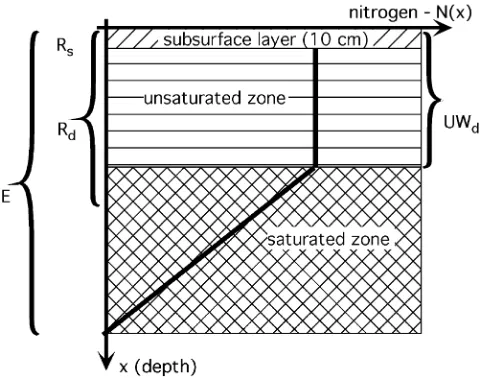
The amount of nutrients used for plant growth is in proportion to the net primary production (NPP). The nutrients in the surface storage are assumed to be avail-able for plant uptake only when there is water to dissolve them. This water is taken to be surface water (SW), plus water contained in the 10 cm subsurface layer (Rs in

Fig. 2).

The amount of water in the subsurface layer is

Sr⫽

再

UW·Rs/ UWd, if Rs⬍UWd

UW⫹S·(Rs⫺UWd) / (E⫺UWd), if Rs⬎UWd

;

where UW is the water in the unsaturated storage, S is saturated water, Rs is the depth of the subsurface layer

(Rs=10 cm), UWdis the unsaturated layer depth and E

is elevation at the given locality. The total amount of

Fig. 2. Calculations of nutrients in the sediment available for root uptake. A linear decline in nutrient concentrations is assumed. E is the elevation, Rdis the root zone depth, Rsis the depth of the subsurface layer associated with the surface water flow, UWdis the depth of the unsaturated layer.

water available to dissolve the nutrients is SW + Srand

the concentration of nutrients is n Csf =n SW / (SW +

Sr). The amount of nutrients available for plant uptake

is then equal to the total amount of nutrients on the sur-face, when surface water is present, or is represented by only a part of n SW that is estimated to be in the subsurface storage:

n Asw⫽

再

n Csw·(SW⫹Sr)⫽n SW, if SW⬎0

n Csw·(1⫺n Dd)·Sr, if SW⫽0

.

The coefficient n Dd is used to separate between the

amount of nutrients that are dissolved and further infil-trated into groundwater and the nutrients that are retained in the subsurface layer (Rs).

Then for the uptake of nutrients from the surface we may assume the rate:

n SWup⫽min(n Asw, n Usw·NPP),

where NPP is the net primary production of plants calcu-lated in the plants module, and n Usw is the parameter

for nutrient requirements of photosynthesis.

The description of nutrients uptake from the sediment (both unsaturated plus saturated zone) is more compli-cated, since we need to parameterize the gradual decrease of nutrient concentration with depth (Fig. 2), also taking into account the depth of the root zone. Assuming that the concentration of nutrients is the same throughout the unsaturated zone and then decreases to zero at the bottom of the elevation considered, we may

write that n S =

冕

E

R_s

N(x)dx, where N(x) is the vertical

the amount of nutrients available for uptake in the root

zone Rdis n S(y)=

冕

R_s

N(x)dx. Therefore the amount of

nutrients available for plant uptake in the sediment is:

n As⫽

冦

0, if RdⱕRs

n S·(2E⫺UWd⫺Rd)(Rd⫺Rs)

(E⫺Rd)(E⫺UWd)

, if Rd⬎RsⱖUWd

n S·2(Rd⫺Rs) / (E⫺Rs), if Rs⬍Rd⬍UWd

n S

E⫹UWd⫺2Rs

·

冉

(2E⫺UWd⫺Rd)(Rd⫺UWd)

E⫺UWd

冊

, otherwise

Here Rdis the root depth calculated in the plants module.

The uptake of nutrients from the sediment is then similar to the one calculated for the surface:

n SDup⫽min(n As, n Us·NPP)

where n Us is the uptake parameter for the sediment

storage of nutrients. In all the above formulas, n = N or P for nitrogen or phosphorus, respectively.

5.4. Vertical transport

Nutrients are dissolved in water and carried with hydrologic flows, both in the vertical and horizontal dimensions. The downflow from n SW to n S is asso-ciated with the infiltration of water from the surface into the sediment:

N⫽n Csw·n Dd·(UWp⫹Sp⫹SW S),

where n Cswis the nutrient concentration on the surface,

n Ddis the separation coefficient discussed above, UWp

and Sp are the amount of rainfall infiltrated into

unsatu-rated storage and satuunsatu-rated storage, respectively, and SW S is the flow from surface water into the saturated storage. The reverse process occurs when saturated water hits the surface and flows out:

Nup⫽n Cs·S SW,

where n Cs is the nutrient concentration in the

sedi-ment, n Cs=n S / (S + SW), and S SW is the flow from

saturated storage to the surface. Both S SW and SW S flows are calculated in the hydrologic module.

5.5. Sorption

At higher concentrations, PO4 becomes adsorbed by

organic material and metal ions in the soil. The rate of sorption is controlled by the amount of organic material in the soil. At lower concentrations of soluble PO4 in

the sediment, P SS becomes available again and returns back into the nutrient cycle.

5.6. Spatial implementation

The horizontal spatial fluxes of nutrients are closely tied to the hydrologic flows. Therefore they are

described together with the hydrologic flows on the sur-face (SWTRANS1 and SWTRANS2), and in the ground (GWTRANS).

6. Plants

6.1. State variables

In the plant module, we simulate the growth of higher vegetation. It will be the macrophytes in an aquatic environment, trees in forests, crops in agricultural habi-tats, grasses and shrubs in grasslands. The plant biomass (kg/m2_{) is assumed to consist of the photosynthetic (PH)}

and the non-photosynthetic (NPH) components. In addition to that we distinguish between the above ground and the below ground biomasses (Fig. 3).

Another state variable (Bt) is employed to track the

so-called biological time in the module. Biological time is the sum of effective daily average temperatures over the life span of the plant (growing degree-days). The temperature is called effective if it exceeds a certain value (5°C in our case). These are the temperatures that are most suitable for the physiological development of the plant. Therefore the total of such temperatures is a good indicator of the plant life stage and may be used to trigger certain processes such as sprouting and appear-ance of reproductive organs.

The module imports temperature and solar radiation data from the physical module, nutrient availability from the nutrient modules, and water availability from the hydrologic module.

6.2. Temperature limitation

There are a great variety of functions that can be used to represent the temperature (T) limitation Lton growth

processes (Jorgensen, 1980). In most cases, a bell-shaped

curve is described, which has a range of optimal tem-peratures where the limitation is negligible (Lt = 1)

whereas at other temperatures, the growth slows down or stops completely (Lt ⬎0).

This behavior is provided by a function described by

Lassiter and Kearns (1974):

Lt⫽exp(s1·(T⫺Topt))·

冉

Tmax⫺T

Tmax⫺Topt

冊

s₁(T_max⫺T_opt)

.

Here, Topt is the optimal temperature, Tmax is the

maxi-mal temperature after which the growth stops, s1 is the

curvature parameter that regulates the form of the curve. Another function (Voinov and Akhremenkov, 1990) that is more complex, but offers more flexibility in defining the shape of the temperature limitation curve is:

Lt ⫽

冦

f(1⫺T/T_max)s1

0 , if T⬍Topt

f

冉

T_max⫺T T_max⫺T_opt

冊

s₁

m , otherwise

where the additional parameters are f0 the value of the

function at zero temperature (Lt(0) = f0); and fm the

value of the function at maximal temperature (Lt(Tmax) = fm).

6.3. Light limitation

Another factor that limits photosynthesis is the avail-ability of light. The light limitation (Li) is defined as:

Li⫽

I Is

exp

冉

冊

,

where I is the incoming solar radiation, and Is is the

saturation level for irradiation.

6.4. Water limitation

If there is too much or too little water, the process of plant growth slows down. To account for the deficit of water, the function W0 (Fig. 4) is used.

W0 ⫽ sin(Wa·π/ 2)m,

where Wa is the available water, m is the water deficit

tolerance coefficient. When the tolerance is high (m ⬍ 1), the plant can grow fast enough even under low water availability. When tolerance is low (m1), the plant growth declines whenever water availability becomes below 1.

As with inadequate water availability, excess water may also be detrimental to plant growth. Certain plants require that a proportion of the root zone be above the water table to ensure that there is no limitation. Other plants grow well as long as they are covered by surface

Fig. 4. General form of limitation function used for water avail-ability. (a) m=0.5; (b) m=2.0; (c) m=5.0.

water to a certain level, but then if there is more water, their growth becomes inhibited. The function W1 is to

take into account both conditions. The coefficient k the tolerance to high water stage represents the tolerance to surface water stage when it is negative, and represents the requirement of a proportion of the root zone to be above the water table when it is positive:

W1⫽

冦

1 / (1⫹exp(SW⫹k)), if k⬍0傼SW⬎ ⫺k;

min(1,UW / Rd/ k), if k ⬎0傼Rd⬎0;

1, otherwise

Here SW is the surface water, UW is the water in the unsaturated storage, and Rdis the root depth. As the

sur-face water stage exceeds the tolerance level, or the unsaturated depth becomes less than Rd·k, W1 becomes

smaller than 1 and limits the plant growth.

The overall water limitation (0 ⬍ Lw ⬍ 1) is then

calculated as Lw= min(W0,W1).

6.5. Nutrient limitation

The standard Michaelis–Menten equation is assumed to calculate the uptake (fn) of each individual nutrient:

fn⫽Sn/ (Sn⫹Cn),

where Snis the nutrient ambient concentration, Cnis the

Ln ⫽ min(fN, fP).

6.6. Net primary production

The four limiting functions for light, temperature, moisture and nutrient availability are assumed to be multiplicative. The NPP is then calculated as

FNPP⫽anpp·Lt·Li·Lw·Ln·PH·(1⫺PH / PHM),

where anpp is the photosynthesis rate (1/day), and PHM

is the maximal photosynthetic biomass for the given type of plant.

6.7. Planting

Some types of plants, such as agricultural crops, are planted at a certain time, tP. During planting, a given

amount of biomass is introduced into the system and then starts to grow. If seeds are planted, then the biomass introduced is non-photosynthetic. This biomass remains inactive until the biological time Btbecomes larger than

a certain threshold Bst. After that, the translocation

pro-cess described below starts to channel the biomass from the non-photosynthetic (NPH) to the photosynthetic (PH) storage. As PH appears, photosynthesis begins and the plant starts to grow.

6.8. Translocation

We describe the distribution of new biomass among the model compartments based on the following two pro-portions: a∗ =max(a) = max(PH / BMa) the maximum

ratio of photosynthetic biomass to above ground biomass (BMa); and b=NPHa/ NPHb the ratio of above ground

non-photosynthetic biomass (NPHa) to below ground

non-photosynthetic biomass (NPHb), which is assumed

to be constant.

Using these two ratios, we can calculate most of the other model fluxes and compartments. The above ground non-photosynthetic biomass is NPHa = bNPH / (1 + b),

and the below ground component is NPHb = NPH / (1 + b). When there is more photosynthetic biomass pro-duced than transferred into the non-photosynthetic stor-age, then a ⬎ a∗. During periods that are unfavorable for photosynthetic production, a may become small, a

⬍a∗. However, at all times, the plant is assumed to try and maximize photosynthetic biomass,a=a∗. The two processes that are employed for this purpose are Transup and Transdown. Transup describes the translocation of material from the non-photosynthetic storage (roots, branches) into the photosynthetic parts of the plant (leaves), and dominates at the start of the growth period or during periods unfavorable for growth when stored assimilates are used to maintain plant growth. Recipro-cally, the Transdown dominates during periods of effec-tive photosynthesis, when more assimilates are produced

than currently needed and a portion can be channeled into storage in the non-photosynthetic parts of the plant. In both cases, the plant tries to maintain the proportion between the photosynthetic and non-photosynthetic parts as close to a∗as possible.

The above ground biomass BMa = PH + NPHa =

PH +bNPH / (1 +b).

Therefore a = PH / [PH + bNPH / (1 + b)], and the translocation mechanism should operate is such a way that a→a∗. This condition is altered for certain plants

that grow reproductive organs (such as crops). As soon as the reproduction process comes into play, the plant changes the translocation patterns and growth of the reproductive organs becomes a priority. Since we do not have a special variable to account for these organs, we assume that they are part of the non-photosynthetic stor-age and when biological time exceeds the threshold for reproduction, the translocation is altered in favor of the NPH stock.

The proportion of the newly produced photosynthetic material that is translocated into the non-photosynthetic storage is then described as:

T-⫽

冦

cos((π/ 2)a∗/a), ifa⬎a∗

1⫺1 / Bt, if Bt⬎br

0, otherwise

where br is the biological time threshold after which

reproductive organs start to develop.

The reverse process of translocation from the non-photosynthetic storage to generate photosynthetic biomass, Transup, occurs at the beginning of the veg-etation period and is also triggered by the biological time counter Bt.

6.9. Mortality, litterfall and harvest

These three flows occur at different times but they all decrease the plant biomass. Mortality is a natural process of decay of certain plant parts that is assumed to occur at a constant rate as a proportion of the photosynthetic and non-photosynthetic biomasses.

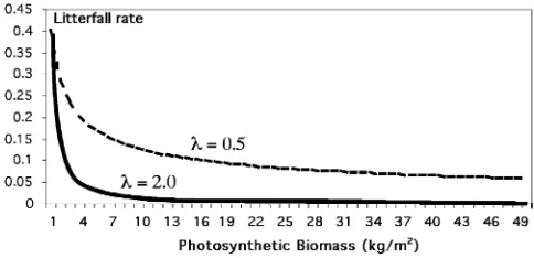
Deciduous plants shed their leaves (PH biomass) in the fall. The process is triggered by changes in day length: once day length becomes smaller than a certain threshold value, the litterfall process starts. The litterfall process starts slow and then accelerates as less photosyn-thetic biomass is left:

FL⫽

冦

0, if D⬎dl兩DⱖD(t⫺1)

PH, if PH⬍pmin

Here, the first condition only allows litterfall to occur in fall when the day length D is decreasing and becomes less than the threshold value dl. The second condition

clears the foliage completely after a certain minimal biomass pminis reached. The third condition is the

grad-ual litterfall that starts when the day length requirement is reached; l is the litterfall rate and n is the intensity (n = 3); PHmaxis the maximal biomass reached during

the season. It serves as a reference point from which to decrease the photosynthetic biomass (Fig. 5).

The harvest is another process that removes plant biomass. At harvest time, tH, certain proportions of PH

and NPH are taken out of the system. Right after harvest occurs, a certain portion, r, of the biomass left, is made available for the mortality flows that quickly channel the living biomass into the dead organic pool and make it available for decomposition. For seasonal crops, r= 1, and all the biomass remaining after harvest rapidly dies off. For perennial crops,r→0, and there is no additional mortality caused by the harvest.

6.10. Spatial implementation and crop rotation

The spatial distribution of plants is fixed; plants do not travel horizontally in the landscape. Therefore the only spatial changes that can occur to the vegetation are connected to human activities, such as crop rotation, or other management practices. The spatial module that takes care of crop rotation is called by CROPROT (HAB MAP, DAYJUL), where DAYJUL is the Julian day, and HAB MAP is the Habitat map of the area. The function scans the whole area and switches land use type from one to another according to the current land use and the Julian day. The sequence of crops is fixed and is determined by the matrix (Fig. 6) where each crop is associated with a certain time interval. For each of the cells (i,j) and each of the crops, we perform the oper-ation:

if(TIME⫽ ⫽TIMEk& HAB MAP(i,j)⫽

⫽CROPk⫺1)HAB MAP(i,j)⫽CROPk

where TIMEkis the planting day for CROPk.

Fig. 5. Litterfall function. As the remaining photosynthetic biomass PH decreases the rate of litterfall increases.

7. Detritus

7.1. State variables

At present, this module serves predominantly to close the nutrient and material cycles in the system, it does not go into all the details of the multi-scale and complex processes of leaching and bacterial decomposition. As biomass dies off, part of it turns into stable detritus, DS,

whereas the rest becomes labile detritus, DL. The

pro-portions between the two are driven by the lignin con-tent, which is relatively low for the PH biomass and is quite high for NPH biomass. Labile detritus is decom-posed directly, and stable detritus is decomdecom-posed either to labile detritus, or becomes deposited organic material (DOM), DDOM.

7.2. Decomposition

Avoiding much of the complexities, we assume the decomposition process as linear. The decay of stable detritus is

FDS⫽d0·DS⫹d1·LDT·DS,

where d0is the flow rate of stable detritus transformation

into DDOM, d1 is the flow rate between stable and labile

detritus. The latter flow is modified by Vant-Hoff tem-perature limitation function LDT =2(T⫺20) / 10, where T is

the ambient air temperature (°C). The decomposition of labile detritus and DOM are described similarly as linear functions modified by the Vant-Hoff temperature func-tion.

8. Calibration and test runs

We have been mostly using the LHEM for modeling of the Patuxent watershed as well as several of its sub-watersheds. Another watershed that was modeled is the Gwynns Falls, a highly urbanized watershed in Balti-more. The details of the PLM and its results have been reported elsewhere (Voinov et al., 1999a; Costanza et al., 2002), and may also be found at

http://giee.uvm.edu/PLM. This brief description of the

multi-Fig. 6. Diagram of crop rotation most commonly implemented in Maryland. A user code modifies the Habitat Map used in the model according to this rotation. As a result, the modules get different sets of habitat dependent parameters at different times of the year.

tier calibration method, described by Voinov et al.

(1999a). The calibration of the full model has been

achi-eved in a step-wise process that started with the cali-bration of individual modules, moving then to spatial implementations of modules and groups of modules at several scales, until finally the full ecological model was calibrated for the whole watershed. The obvious benefit of this was a much simpler model to calibrate at each step. Clearly, the aggregate of several modules does not necessarily behave similarly to the individual modules taken separately. Therefore recalibration was needed every time we went from simple individual modules to their combinations, both locally and spatially. However, it was always much easier to fine-tune the already per-forming modules, than to do a full-scale calibration of the full model in its overall complexity.

We started with calibrations of the local hydrologic model. The input from other modules, primarily plants was imitated by fixed time series. For example, a time series was generated to represent the approximate dynamics of plants over a one-year time period. The model produced clearly different dynamics with and without plants (Fig. 7). Adequate data for local hydrologic calibrations was unavailable, since these pro-cesses are essentially spatial and it is hard to localize them and consider outside of the spatial context. There-fore the local hydrology was calibrated only in a “ball-park” fashion to make sure that the model behaves in a stable way in a variety of conditions. Similarly, we could provide only limited calibration of the local nutrient dynamics. This stage of local calibration was important to make sure that all the major fluxes, such as evapor-ation, transpirevapor-ation, percolevapor-ation, nutrient loading, and uptake, are within some reasonable values, that there are no inexplicable trends in the model. It was also important to run the sensitivity analysis and understand the effect of individual parameters on overall dynamics. Most of the calibrations for these modules were done in combination with the module for spatial dynamics added within the SME context. The spatial model for hydrology and nutrients, or the water quality model has been calibrated for several subwatersheds in the Patux-ent. We identified two spatial scales at which to run the model a 200 m and 1 km cell resolution. The 200 m

Fig. 7. Local hydrology dynamics with (A) and without (B) plant biomass considered. There is a clear effect of transpiration upon the amount of water in the unsaturated and saturated storage. When plants are present, they increase water storage capacity in the unsaturated layer and consequently higher infiltration rates can also mitigate the worst peak flows of surface water.

resolution was more appropriate to capture some of the ecological processes associated with landuse change but was too detailed and required too much computer pro-cessor time to perform the numerous model runs required for calibration and scenario evaluation. The 1 km resolution reduced the total number of model cells in the watershed from 58,905 to 2352 cells.

We did most of the preliminary calibrations for a small (23 km2

sub-watershed that of Hunting creek, was located in the southern part of Patuxent, quite different in terms of soils and elevations. It also included an estuarine part that allowed us to test the second hydrologic algorithm that was designed for open water. The next larger watershed was the upper non-tidal half of the Patuxent watershed that drained to the USGS gage at Bowie (940 km2_{). And}

finally we examined the whole Patuxent watershed (2352 km2

).

We staged additional experiments with the small Hunting creek subwatershed to test the sensitivity of the surface water flux. Three crucial parameters controlled surface flow in the model: infiltration rate, horizontal conductivity and the horizontal flow rate defined by path length on the link map over which water can travel per time step of the unit model. Riverflow peak height was strongly controlled by the infiltration rate. The conduc-tivity determined river levels between storms and the link length modified the width of the storm peaks.

The results of surface water flow calibration have been reported elsewhere (Voinov et al., 1999a, b). They were in good agreement with the gage data, and what is most important, led us to several control parameters that were crucial to modify the patterns of the hydrographs in the way we needed. Whereas some individual peaks and situations were not always reproduced, the model worked well to represent the overall trends in the hydrologic patterns and gave a good estimate of the total outflow dynamics from the area. Spatial nutrient dynam-ics were calibrated for data at several gaging stations on the Patuxent. Fig. 8 displays the calibration results for nitrogen concentrations measured at the USGS station at Bowie, which is in the mid-Patuxent watershed and accounts for dynamics in the upper half of the study area. In contrast to water quality modeling, the plant

mod-Fig. 8. Spatial calibration of the water quality model for the gaging station at Bowie. The data available are quite sporadic and show considerable variability. It is not clear when the measurements were taken and how well they track the peak flows, when the nutrient content is the highest. Nevertheless, the model well represents the general trend and stays within the ranges of variations in the observed data.

ule is less dependent upon spatial interactions. Therefore the unit model calibration in this case is more important. The calibrations were carried out for a series of para-meter sets, representing the different habitat types and plant communities associated with them. We have con-sidered a forest habitat, and a number of agricultural habitats, such as, corn, winter wheat, soybeans and fal-low.

The data set that we used to calibrate the forest dynamics came from field monitoring over a 10-year time period at 12 forested sites located within the East-ern United States (Johnson and Lindberg, 1992). This provided mean flux rates and organic matter nutrient contents. Biomass and species composition were derived through the Forest Inventory and Analysis Database (FIA). The forest association used to select data was oak-hickory with 0.6% coniferous trees. For agricultural habitats, we have used data from the Maryland Cooper-ative Extension Agricultural Nutrient Management

Pro-gram (http://www.agnr.umd.edu/users/agron/nutrient/

home.html#homeplace), and other sources (Schroder et

al., 1995).

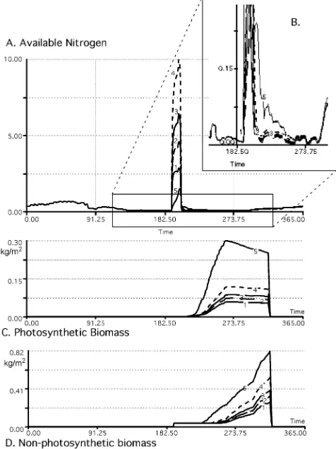
It was most important to make sure that the available parameter set was sufficient to represent a variety of plant behaviors for different habitats and control factors. The overall pattern of growth, maturity and decay is similar for most of the plants; however, the dynamics of photosynthetic and non-photosynthetic biomasses varies for different plants. In Fig. 9, we represent the various growth curves for different habitats. The module produc-ing these curves was the same plant module described above, only the parameter sets were different.