Similarity Learning via Kernel Preserving Embedding

The Thirty-Third AAAI Conference on Artificial Intelligence (AAAI-19)

Similarity Learning via Kernel Preserving Embedding

Zhao Kang,

Yiwei Lu,

_{Yuanzhang Su,}

_{Changsheng Li,}

_{Zenglin Xu}

1_{School of Computer Science and Engineering, University of Electronic Science and Technology of China, China} 2_{Department of Computer Science, University of Manitoba, 66 Chancellors Cir, Winnipeg, MB R3T 2N2, Canada} 3_{School of Foreign Languages, University of Electronic Science and Technology of China, Sichuan 611731, China} [email protected], [email protected], [email protected], [email protected], [email protected]

Abstract

Data similarity is a key concept in many data-driven applica-tions. Many algorithms are sensitive to similarity measures. To tackle this fundamental problem, automatically learning of similarity information from data via self-expression has been developed and successfully applied in various models, such as low-rank representation, sparse subspace learning, semi-supervised learning. However, it just tries to reconstruct the original data and some valuable information, e.g., the mani-fold structure, is largely ignored. In this paper, we argue that it is beneficial to preserve the overall relations when we ex-tract similarity information. Specifically, we propose a novel similarity learning framework by minimizing the reconstruc-tion error of kernel matrices, rather than the reconstrucreconstruc-tion error of original data adopted by existing work. Taking the clustering task as an example to evaluate our method, we ob-serve considerable improvements compared to other state-of-the-art methods. More importantly, our proposed framework is very general and provides a novel and fundamental build-ing block for many other similarity-based tasks. Besides, our proposed kernel preserving opens up a large number of possi-bilities to embed high-dimensional data into low-dimensional space.

Introduction

Nowadays, high-dimensional data can be collected every-where, either by low-cost sensors or from the internet (Chen et al. 2012). Extracting useful information from massive high-dimensional data is critical in different areas like text, images, videos and more. Data similarity is especially im-portant since it is the input for a number of data anal-ysis tasks, such as spectral clustering (Ng et al. 2002; Chen et al. 2018), nearest neighbor classification (Wein-berger, Blitzer, and Saul 2005), image segmentation (Li et al. 2016), person re-identification (Hirzer et al. 2012), im-age retrieval (Hoi, Liu, and Chang 2008), dimension re-duction (Passalis and Tefas 2017), and graph-based semi-supervised learning (Kang et al. 2018a). Therefore, similar-ity measure is crucial to the performance of many techniques and is a fundamental problem in machine learning, pattern recognition, and data mining communities (Gao et al. 2017;

∗

Corresponding author.

Copyright c2019, Association for the Advancement of Artificial Intelligence (www.aaai.org). All rights reserved.

Towne, Ros´e, and Herbsleb 2016). A variety of similar-ity metrics, e.g., Cosine, Jaccard coefficient, Euclidean dis-tance, Gaussian function, are often used in practice for convenience. However, they are often data-dependent and sensitive to noise (Huang, Nie, and Huang 2015). Conse-quently, different metrics lead to a big difference in the final results. In addition, several other similarity measure strategies are popular in dimension reduction techniques. For example, in the widely used locally linear embedding (LLE) (Roweis and Saul 2000), isomeric feature mapping (ISOMAP) (Tenenbaum, De Silva, and Langford 2000), and locality preserving projection (LPP) (Niyogi 2004) methods, one has to construct an adjacency graph of neighbors. Then, k-nearest-neighborhood (knn) and -nearest-neighborhood graph construction methods are often utilized. These ap-proaches also have some inherent drawbacks, including 1) how to determine neighbor numberkor radius; 2) how to choose an appropriate similarity metric to define neighbor-hood; 3) how to counteract the adverse effect of noise and outliers; 4) how to tackle data with structures at different scales of size and density. Unfortunately, all these factors heavily influence the subsequent tasks (Kang et al. 2018b).

Recently, automatically learning of similarity information from data has drawn significant attention. In general, it can be classified into two categories. The first one is adaptive neighbors approach. It learns similarity information by as-signing a probability for each data point as the neighborhood of another data point (Nie, Wang, and Huang 2014). It has been shown to be an effective way to capture the local man-ifold structure.

The other one is self-expression approach. The basic idea is to represent every data point by a linear combination of other data points. In contrast, LLE reconstructs the original data by expressing each data point as a linear combination of itsknearest neighbors only. Through minimizing this re-construction error, we can obtain a coefficient matrix, which is also named similarity matrix. It has been widely applied in various representation learning tasks, including sparse subspace clustering (Elhamifar and Vidal 2013; Peng et al. 2016), low-rank representation (Liu et al. 2013), multi-view learning (Tao et al. 2017), semi-supervised learning (Zhuang et al. 2017), nonnegative matrix factorization(NMF) (Zhang et al. 2017).

origi-nal data and has no explicit mechanism to preserve manifold structure information about the data. In many applications, the data can display structures beyond simply being low-rank or sparse. It is well-accepted that it is essential to take into account structure information when we perform high-dimensional data analysis. For instance, LLE preserves the local structure information.

In view of this issue with the current approaches, we pro-pose to learn the similarity information through reconstruct-ing the original data kernel matrix, which is supposed to preserve overall relations. By doing so, we expect to ob-tain more accurate and complete data similarity. Consider-ing clusterConsider-ing as a specific application of our proposed sim-ilarity learning method, we demonstrate that our framework provides impressive performance on several benchmark data sets. In summary, the main contributions of this paper are threefold:

• Compared to other approaches, the use of the kernel-based distances allows to work on preserving the sets of overall relations rather than individual pairwise similari-ties.

• Similarity preserving provides a fundamental build-ing block to embed high-dimensional data into low-dimensional latent space. It is general enough to be ap-plied to a variety of learning problems.

• We evaluate the proposed approach in the clustering task. It shows that our algorithm enjoys superior performance compared to many state-of-the-art methods.

Notations. Given a data set {x1, x2,· · · , xn}, we denote

X ∈ Rm×n _{with m features and n instances. Then the}

(i, j)-th element of matrixX are denoted by xij. The `2 -norm of a vector x is represented by kxk = √xT _·x,

whereT denotes transpose. The`1-norm of X is defined askXk1 =Pij|xij|. The squared Frobenius norm is

rep-resented as kXk2

F =

P

ijx

2

ij. The nuclear norm of X

is kXk∗ = Pσi, where σi is the i-th singular value of

X. I is the identity matrix with a proper size. ~1 repre-sents a column vector whose every element is one.Z ≥0

means all the elements ofZ are nonnegative. Inner product < xi, xj >=xTi ·xj.

Related Work

In this section, we provide a brief review of existing auto-matic similarity learning techniques.

Adaptive Neighbors Approach

In a similar spirit of LPP, for each data pointxi, all the data

points{xj}nj=1can be regarded as the neighborhood ofxi

with probabilityzij. To some extent,zij represents the

sim-ilarity between xi andxj (Nie, Wang, and Huang 2014).

The smaller distancekxi−xjk2is, the greater the

probabil-ityzijis. Rather than prespecifyingZwith the deterministic

neighborhood relation as LPP does, one can adaptively learn

Zfrom the data set by solving an optimization problem:

min

zi n

X

j=1

(kxi−xjk2zij+αzij2)s.t. zTi~1 = 1, 0≤zij ≤1,

(1) whereαis the regularization parameter. Recently, a variety of algorithms have been developed by using Eq. (1) to learn a similarity matrix. Some applications are clustering (Nie, Wang, and Huang 2014), NMF (Huang et al. 2018), and fea-ture selection (Du and Shen 2015). This approach can effec-tively capture the local structure information.

Self-expression Approach

The so-called self-expression is to approximate each data point as a linear combination of other data points, i.e.,xi=

P

jxjzij. The rationale here is that ifxi andxj are

simi-lar, weightzijshould be big. Therefore,Zalso behaves like

the similarity matrix. This shares the similar spirit as LLE, except that we do not predetermine the neighborhood. Its corresponding learning problem is:

min

Z

1

2kX−XZk

2

F+αρ(Z) s.t. Z ≥0, (2)

whereρ(Z)is a regularizer ofZ. Two commonly used as-sumptions aboutZare low-rank and sparse. Hence, in many domains, we also callZas the low-dimensional representa-tion ofX. Through this procedure, the individual pairwise similarity information hidden in the data is explored (Nie, Wang, and Huang 2014) and the most informative “neigh-bors” for each data point are automatically chosen.

Moreover, this learned Z can not only reveal low-dimensional structure of data, but also be robust to data scale (Huang, Nie, and Huang 2015). Therefore, this approach has drawn significant attention and achieved impressive perfor-mance in a number of applications, including face recog-nition (Zhang, Yang, and Feng 2011), subspace clustering (Liu et al. 2013; Elhamifar and Vidal 2013), semi-supervised learning (Zhuang et al. 2017). In many real-world applica-tions, data often present complex structures. Nevertheless, the first term in Eq. (2) simply minimizes the reconstruction error. Some important manifold structure information, such as overall relations, could be lost during this process. Pre-serving relation information has been shown to be important for feature selection (Zhao et al. 2013). In (Zhao et al. 2013), new feature vector f is obtained by maximizing fT_{Kfˆ ,}

whereKˆ is the refined similarity matrix derived from origi-nal kernel matrixKwith elementK(x, y) =φ(x)Tφ(y). In this paper, we propose a novel model to preserve the overall relations of the original data and simultaneously learn the similarity matrix.

Proposed Methodology

finding a new representation which preserves overall rela-tions as much as possible.

Given a data matrixX, one of the most commonly used relation measures is the inner product. Specifically, we try to minimize the inconsistency between two inner products: one for the raw data and another for reconstructed dataXZ. To make our model more general, we build it in a transformed space,i.e.,Xis mapped byφ(Xu et al. 2009). We have

min

Z kφ(X) T

·φ(X)−(φ(X)Z)T ·(φ(X)Z)k2F (3)

(3) can be simplified as

min

Z kK−Z T_KZk2

F. (4)

With certain assumption about the structure of Z, our proposed Similarity Learning via Kernel preserving

Embedding (SLKE) framework can be formulated as

min

Z

1

2kK−Z

T_KZk2

F +γρ(Z) s.t. Z ≥0, (5)

whereγ >0is a tradeoff parameter andρis a regularizer on Z. If we use the nuclear normk · k∗to replaceρ(·), we have

a low-rank representation. If the`1-norm is adopted, we ob-tain a sparse representation. It is worth pointing out that Eq. (5) enjoys several nice properties:

1) The use of kernel-based distance preserves the sets of overall relations, which will benefit the subsequent tasks; 2) This learned low-dimensional representation or similarity matrixZ is general enough to be utilized to solve a variety of different tasks, where similarity information is needed; 3) The learned representation is particularly suitable to prob-lems that are sensitive to data similarity, such as clustering (Kang et al. 2018c), classification (Wright et al. 2009), rec-ommender systems (Kang, Peng, and Cheng 2017a); 4) Its input is the kernel matrix. This is also desirable, as not all types of data can be represented in numerical fea-ture vectors form (Xu et al. 2010). For instance, we need to group proteins in bioinformatics based on their structures and to divide users in social media based on their friendship relations.

In the following section, we will show a simple strategy to solve problem (5).

Optimization

It is easy to see that Eq. (5) is a fourth-order function ofZ. Directly solving it is not so straightforward. To circumvent this problem, we first convert it to the following equivalent problem by introducing two more auxiliary variables

min

Z

1 2kK−J

T_KWk2

F +γρ(Z)

s.t. Z≥0, Z=J, Z=W.

(6)

Now we resort to the alternating direction method of mul-tipliers (ADMM) method to solve (6). The corresponding augmented Lagrangian function is:

L(Z, J, W, Y1, Y2) =

1 2kK−J

T_KWk2

F+γρ(Z)+

µ

2

kZ−J+Y1

µk

2

F+kZ−W +

Y2

µk

2

F

,

(7)

whereµ >0is a penalty parameter andY1,Y2are the la-grangian multipliers. The variablesZ,W, andJcan be up-dated alternatingly, one at each step, while keeping the other two fixed.

To solveJ, we observe that the objective function (7) is a strongly convex quadratic function inJwhich can be solved by setting its first derivative to zero, we have:

J = (µI+KW WTKT)−1(µZ+Y1+KW KT), (8) whereI∈ Rn×n_{is the identity matrix.}

Similarly,

W = (µI+KTJ JTK)−1(µZ+Y2+KTJ K). (9) ForZ, we have the following subproblem:

min

Z γρ(Z) +µ

Z−J+W−

Y1+Y2

µ

2

2

F

. (10)

Depending on different regularization strategies, we have different closed-form solutions for Z. Define H =

J+W−Y1 +Y2

µ

2 , we can write its singular value decomposition (SVD) asU diag(σ)VT_{. Then, for low-rank representation,}

i.e.,ρ(Z) =kZk∗, we have,

Z=U diag(max{σ− γ

2µ,0})V

T_{. (11)}

For sparse representation, i.e.,ρ(Z) =kZk1, we can up-dateZelement by element as,

Zij=max{|Hij| −

γ

2µ,0} ·sign(Hij). (12) For clarity, the complete procedures to solve the problem (5) are outlined in Algorithm 1.

Algorithm 1:The algorithm of SLKE

Input:Kernel matrixK, parametersγ >0,µ >0.

Initialize:Random matrixW andZ,Y1=Y2= 0.

REPEAT

1: CalculateJby (8).

2: UpdateW according to (9). 3: CalculateZusing (11) or (12).

4: Update Lagrange multipliersY1andY2as

Y1=Y1+µ(Z−J),

Y2=Y2+µ(Z−W).

UNTILstopping criterion is met.

Complexity Analysis

With our optimization strategy, the complexity for J is

O(n3_{). Updating W has the same complexity as J. Both}

its complexity isO(n3). Since we seek a low-rank matrix and so only need a few principle singular values. Package like PROPACK can compute a rankkSVD with complex-ityO(n2_{k)(Larsen 2004). To obtain a sparse solution ofZ,} we needO(n2_{)complexity. The updating ofY}

1andY2cost

O(n2).

Experiments

To assess the effectiveness of our proposed method, we ap-ply the learned similarity matrix to do clustering.

Data Sets

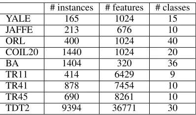
Table 1: Description of the data sets

# instances # features # classes

YALE 165 1024 15

JAFFE 213 676 10

ORL 400 1024 40

COIL20 1440 1024 20

BA 1404 320 36

TR11 414 6429 9

TR41 878 7454 10

TR45 690 8261 10

TDT2 9394 36771 30

We conduct our experiments with nine benchmark data sets, which are widely used in clustering experiments. We show the statistics of these data sets in Table 1. In summary, the number of data samples varies from 165 to 9,394 and feature number ranges from 320 to 36,771. The first five data sets are images, while the last four are text data.

Specifically, the five image data sets contain three face databases (ORL, YALE, and JAFFE), a toy image database COIL20, and a binary alpha digits data set BA. For example, COIL20 consists of 20 objects and each object was taken from different angles. BA data set contains images of dig-its of “0” through “9” and letters of capital “A” through “Z”. YALE, ORL, and JAFEE consist of images of the per-son. Each image represents different facial expressions or configurations due to times, illumination conditions, and glasses/no glasses.

Data Preparation

Since the input for our proposed method is kernel ma-trix, we design 12 kernels in total to fully examine its performance. They are: seven Gaussian kernels of the form K(x, y) = exp(−kx − yk2

2/(td2max)) with t ∈

{0.01,0.05,0.1,1,10,50,100}, where dmax denotes the

maximal distance between data points; a linear kernel K(x, y) = xT_{y; four polynomial kernelsK(x, y) = (a+}

xT_y)b_{of the form witha∈ {0,1}andb ∈ {2,4}. Besides,}

all kernels are rescaled to[0,1]by dividing each element by the largest element in its corresponding kernel matrix. These kernels are commonly used types in the literature, so we can well investigate the performance of our method.

Comparison Methods

To fully examine the effectiveness of the proposed frame-work on clustering, we choose a good set of methods to compare. In general, they can be classified into two categories: similarity-based and kernel-based clustering methods.

• Spectral Clustering (SC)(Ng et al. 2002): SC is a widely used clustering method. It enjoys the advantage of ex-ploring the intrinsic data structures. Its input is the graph Laplacian, which is constructed from the similarity ma-trix. Here, we directly treat kernel matrix as the similar-ity matrix for spectral clustering. For our proposed SLKE method, we employ learnedZ to do spectral clustering. Thus, SC serves as a baseline method.

• Robust Kernel K-means (RKKM)1 _{(Du et al. 2015):} Based on classical k-means clustering algorithm, RKKM has been developed to deal with nonlinear structures, noise, and outliers in the data. RKKM demonstrates su-perior performance on a number of real-world data sets.

• Simplex Sparse Representation (SSR)(Huang, Nie, and Huang 2015): SSR method has been proposed recently. It is based on adaptive neighbors idea. Another appealing property of this method is that its model parameter can be calculated by assuming a maximum number of neigh-bors. Therefore, we don’t need to tune the parameter any more. In addition, it outperforms many other state-of-the-art techniques.

• Low-Rank Representation (LRR) (Liu et al. 2013): Based on self-expression, subspace clustering with low-rank regularizer achieves great success on a number of ap-plications, such as face clustering, motion segmentation.

• Sparse Subspace Clustering (SSC)(Elhamifar and Vi-dal 2013): Similar to LRR, SSC assumes a sparse solu-tion ofZ. Both LRR and SSC learn similarity matrix by reconstructing the original data. In this aspect, SC, LRR, and SSC are baseline methods w.r.t. our proposed algo-rithm.

• Clustering with Adaptive Neighbor (CAN)(Nie, Wang, and Huang 2014). Based on the idea of adaptive neigh-bors, i.e., Eq.(1), CAN learns a local graph from raw data for clustering task.

• Twin Learning for Similarity and Clustering (TLSC)

(Kang, Peng, and Cheng 2017b): Recently, TLSC has been proposed and has shown promising results on real-world data sets. TLSC does not only learn similarity ma-trix via self-expression in kernel space, but also have op-timal similarity graph guarantee. Besides, it has good the-oretical properties, i.e., it is equivalent to kernel k-means and k-means under certain conditions.

• SLKE: Our proposed similarity learning method with overall relations preserving capability. After obtaining similarity matrixZ, we use spectral clustering to conduct clustering experiments. We test both low-rank and sparse

1

regularizer. We denote them as SLKE-R and SLKE-S, re-spectively2_.

Evaluation Metrics

To quantitatively and effectively assess the clustering perfor-mance, we utilize the two widely used metrics (Peng et al. 2018), accuracy (Acc) and normalized mutual information (NMI).

Acc discovers the one-to-one relationship between clus-ters and classes. Letliandˆlibe the clustering result and the

ground truth cluster label ofxi, respectively. Then the Acc

is defined as

Acc=

Pn

i=1δ(ˆli, map(li))

n ,

wherenis the sample size, Kronecker delta functionδ(x, y)

equals one if and only ifx = y and zero otherwise, and map(·) is the best permutation mapping function that maps each cluster index to a true class label based on Kuhn-Munkres algorithm.

Given two sets of clustersLandLˆ, NMI is defined as

NMI(L,Lˆ) =

P

l∈L,ˆl∈Lˆ

p(l,ˆl)log( p(l,ˆl)

p(l)p(ˆl))

max(H(L), H( ˆL)) ,

wherep(l)andp(ˆl)represent the marginal probability distri-bution functions ofLandLˆ, respectively.p(l,ˆl)is the joint probability function ofLandLˆ.H(·)is the entropy func-tion. The greater NMI means the better clustering perfor-mance.

Results

We report the extensive experimental results in Table 2. Except SSC, LRR, CAN, and SSR, we run other methods on each kernel matrix individually. As a result, we show both the best performance among those 12 kernels and the average results over those 12 kernels for them. Based on this table, we can see that our proposed SLKE achieves the best performance in most cases. To be specific, we have the following observations:

1) Compared to classical k-means based RKKM and spectral clustering techniques, our proposed method SLKE has a big advantage in terms of accuracy and NMI. With respect to the recently proposed SSR and TLSC methods, SKLE always obtains better results.

2) SLKE-R and SLKE-S often outperform LRR and SSC, respectively. The accuracy increased by 8.92%, 8.76% on average, respectively. That is to say, kernel-based distance approach indeed performs better than original data recon-struction technique. This verifies the importance of retaining relation information when we learn a low-dimensional rep-resentation, especially for sparse representation.

3) With respect to adaptive neighbors approach CAN, we also obtain better performance on those datasets ex-cept COIL20. For COIL20, our results are quite close to

2

https://github.com/sckangz/SLKE

CAN’s. Therefore, compared to various similarity learning techniques, our method is very competitive.

4) Regarding low-rank and sparse representation, it is hard to conclude which one is better. It totally depends on the specific data.

Furthermore, we run t-SNE (Maaten and Hinton 2008) al-gorithm on the JAFFE data X and the reconstructed data XZfrom the best result of our SLKE-R. As shown by Fig-ure 1, we can see that our method can well preserve the clus-ter structure of the data.

−15 −10 −5 0 5 10 15

−25 −20 −15 −10 −5 0 5 10 15 20 25

1 2 3 4 5 6 7 8 9 10

(a) Original data

−20 −15 −10 −5 0 5 10 15 20

−20 −15 −10 −5 0 5 10 15 20

1 2 3 4 5 6 7 8 9 10

(b) Reconstructed data

Figure 1: JAFFE data set visualized in two dimensions.

(a) Accuracy(%)

Data SC RKKM SSC LRR SSR CAN TLSC SLKE-S SLKE-R

YALE 49.42(40.52) 48.09(39.71) 38.18 61.21 54.55 58.79 55.85(45.35) 61.82(38.89) 66.24(51.28) JAFFE 74.88(54.03) 75.61(67.89) 99.53 99.53 87.32 98.12 99.83(86.64) 96.71(70.77) 99.85(90.89) ORL 58.96(46.65) 54.96(46.88) 36.25 76.50 69.00 61.50 62.35(50.50) 77.00(45.33) 74.75(59.00) COIL20 67.60(43.65) 61.64(51.89) 73.54 68.40 76.32 84.58 72.71(38.03) 75.42(56.83) 84.03(65.65) BA 31.07(26.25) 42.17(34.35) 24.22 45.37 23.97 36.82 47.72(39.50) 50.74(36.35) 44.37(35.79) TR11 50.98(43.32) 53.03(45.04) 32.61 73.67 41.06 38.89 71.26(54.79) 69.32(46.87) 74.64(55.07) TR41 63.52(44.80) 56.76(46.80) 28.02 70.62 63.78 62.87 65.60(43.18) 71.19(47.91) 74.37(53.51) TR45 57.39(45.96) 58.13(45.69) 24.35 78.84 71.45 48.41 74.02(53.38) 78.55(50.59) 79.89(58.37) TDT2 52.63(45.26) 48.35(36.67) 23.45 52.03 20.86 19.74 55.74(44.82) 59.61(25.40) 74.92(33.67)

(b) NMI(%)

Data SC RKKM SSC LRR SSR CAN TLSC SLKE-S SLKE-R

YALE 52.92(44.79) 52.29(42.87) 45.56 62.98 57.26 57.67 56.50(45.07) 59.47(40.38) 64.29(52.87) JAFFE 82.08(59.35) 83.47(74.01) 99.17 99.16 92.93 97.31 99.35(84.67) 94.80(60.83) 99.49(81.56) ORL 75.16(66.74) 74.23(63.91) 60.24 85.69 84.23 76.59 78.96(63.55) 86.35(58.84) 85.15(75.34) COIL20 80.98(54.34) 74.63(63.70) 80.69 77.87 86.89 91.55 82.20(73.26) 80.61(65.40) 91.25(73.53) BA 50.76(40.09) 57.82(46.91) 37.41 57.97 30.29 49.32 63.04(52.17) 63.58(55.06) 56.78(50.11) TR11 43.11(31.39) 49.69(33.48) 02.14 65.61 27.60 19.17 58.60(37.58) 67.63(30.56) 70.93(45.39) TR41 61.33(36.60) 60.77(40.86) 01.16 67.50 59.56 51.13 65.50(43.18) 70.89(34.82) 68.50(47.45) TR45 48.03(33.22) 57.86(38.96) 01.61 77.01 67.82 49.31 74.24(44.36) 72.50(38.04) 78.12(50.37) TDT2 52.23(27.16) 54.46(42.19) 13.09 64.36 02.44 03.97 58.35(46.37) 58.55(15.43) 68.21(28.94)

Table 2: Clustering results obtained on benchmark data sets. The average performance of those 12 kernels is put in parenthesis. The best results among those kernels are highlighted in boldface.

1e−0625 1e−05 0.0001 0.001 0.01 0.1

30 35 40 45 50 55 60

γ

Acc

SKLE-S SKLE-R

(a) Acc

1e−0635 1e−05 0.0001 0.001 0.01 0.1

40 45 50 55 60

γ

NMI

SKLE-S SKLE-R

(b) NMI

Figure 2: The effect of parameterγon the YALE data set.

Table 3: Wilcoxon Signed Rank Test on all Data sets.

Method Metric SC RKKM SSC LRR SSR CAN TLSC

SLKE-S Acc .0039 .0039 .0117 .2500 .0078 .0391 .0391 NMI .0078 .0039 .0195 .6523 .0391 .0547 .3008

Parameter Analysis

In this subsection, we investigate the influence of our model parameterγon the clustering results. Take Gaussian kernel witht = 100of YALE and JAFFE data sets as examples, we plot our algorithm’s performance with γ in the range

[10−6_,10−5_,10−4_,10−3_,10−2_,10−1_{]in Figure 2 and 3,} re-spectively. As we can see that our proposed methods work well for a wide range ofγ, e.g., from10−6_to10−3_.

1e−0650 1e−05 0.0001 0.001 0.01 0.1 60

70 80 90 100

γ

Acc

SKLE-S SKLE-R

(a) Acc

1e−0660 1e−05 0.0001 0.001 0.01 0.1 70

80 90 100

γ

NMI

SKLE-S SKLE-R

(b) NMI

Figure 3: The effect of parameterγon the JAFFE data set.

Conclusion

In this paper, we present a novel similarity learning frame-work relying on an embedding of kernel-based distance. Our model is flexible to obtain either low-rank or sparse repre-sentation of data. Comprehensive experimental results on real data sets well demonstrate the superiority of the pro-posed method on the clustering task. It has great potential to be applied in a number of applications beyond cluster-ing. It has been shown that the performance of the proposed method is largely determined by the choice of kernel func-tion. In the future, we plan to address this issue by

develop-ing a multiple kernel learndevelop-ing method, which is capable of automatically learning an appropriate kernel from a pool of input kernels.

Acknowledgment

This paper was in part supported by Grants from the Natural Science Foundation of China (Nos. 61806045 and 61572111), a 985 Project of UESTC (No. A1098531023601041) and two Fundamental Re-search Fund for the Central Universities of China (Nos. A03017023701012 and ZYGX2017KYQD177).

References

Chen, X.; Ye, Y.; Xu, X.; and Huang, J. Z. 2012. A feature group weighting method for subspace clustering of high-dimensional data. Pattern Recognition45(1):434–446. Chen, X.; Hong, W.; Nie, F.; He, D.; Yang, M.; and Huang, J. Z. 2018. Directly minimizing normalized cut for large scale data. InSIGKDD, 1206–1215.

Du, L., and Shen, Y.-D. 2015. Unsupervised feature selec-tion with adaptive structure learning. InSIGKDD, 209–218. ACM.

Du, L.; Zhou, P.; Shi, L.; Wang, H.; Fan, M.; Wang, W.; and Shen, Y.-D. 2015. Robust multiple kernel k-means using` 2; 1-norm. InIJCAI, 3476–3482. AAAI Press.

Elhamifar, E., and Vidal, R. 2013. Sparse subspace cluster-ing: Algorithm, theory, and applications.IEEE transactions on pattern analysis and machine intelligence35(11):2765– 2781.

Gao, X.; Hoi, S. C.; Zhang, Y.; Zhou, J.; Wan, J.; Chen, Z.; Li, J.; and Zhu, J. 2017. Sparse online learning of image similarity. ACM Transactions on Intelligent Systems and Technology (TIST)8(5):64.

Hirzer, M.; Roth, P. M.; K¨ostinger, M.; and Bischof, H. 2012. Relaxed pairwise learned metric for person re-identification. InECCV, 780–793. Springer.

Hoi, S. C.; Liu, W.; and Chang, S.-F. 2008. Semi-supervised distance metric learning for collaborative image retrieval. In

CVPR, 1–7. IEEE.

Huang, S.; Wang, H.; Li, T.; Li, T.; and Xu, Z. 2018. Robust graph regularized nonnegative matrix factorization for clus-tering. Data Mining and Knowledge Discovery32(2):483– 503.

Huang, J.; Nie, F.; and Huang, H. 2015. A new simplex sparse learning model to measure data similarity for cluster-ing. InIJCAI, 3569–3575.

Kang, Z.; Lu, X.; Yi, J.; and Xu, Z. 2018a. Self-weighted multiple kernel learning for graph-based clustering and semi-supervised classification. InIJCAI, 2312–2318. Kang, Z.; Peng, C.; Cheng, Q.; and Xu, Z. 2018b. Uni-fied spectral clustering with optimal graph. InProceedings of the Thirty-Second AAAI Conference on Artificial Intelli-gence (AAAI-18). AAAI Press.

Kang, Z.; Peng, C.; and Cheng, Q. 2017a. Kernel-driven similarity learning.Neurocomputing267:210–219.

Kang, Z.; Peng, C.; and Cheng, Q. 2017b. Twin learning for similarity and clustering: A unified kernel approach. In Pro-ceedings of the Thirty-First AAAI Conference on Artificial Intelligence (AAAI-17). AAAI Press.

Larsen, R. M. 2004. Propack-software for large and sparse svd calculations.Available online. URL http://sun. stanford. edu/rmunk/PROPACK2008–2009.

Li, T.; Cheng, B.; Ni, B.; Liu, G.; and Yan, S. 2016. Mul-titask low-rank affinity graph for image segmentation and image annotation.ACM Transactions on Intelligent Systems and Technology (TIST)7(4):65.

Liu, G.; Lin, Z.; Yan, S.; Sun, J.; Yu, Y.; and Ma, Y. 2013. Robust recovery of subspace structures by low-rank repre-sentation. IEEE Transactions on Pattern Analysis and Ma-chine Intelligence35(1):171–184.

Maaten, L. v. d., and Hinton, G. 2008. Visualizing data using t-sne. Journal of machine learning research9(Nov):2579– 2605.

Ng, A. Y.; Jordan, M. I.; Weiss, Y.; et al. 2002. On spectral clustering: Analysis and an algorithm.NIPS2:849–856.

Nie, F.; Wang, X.; and Huang, H. 2014. Clustering and projected clustering with adaptive neighbors. InSIGKDD, 977–986. ACM.

Niyogi, X. 2004. Locality preserving projections. InNIPS, volume 16, 153. MIT.

Passalis, N., and Tefas, A. 2017. Dimensionality reduction using similarity-induced embeddings.IEEE transactions on neural networks and learning systems.

Peng, X.; Xiao, S.; Feng, J.; Yau, W.-Y.; and Yi, Z. 2016. Deep subspace clustering with sparsity prior. In IJCAI, 1925–1931.

Peng, C.; Kang, Z.; Cai, S.; and Cheng, Q. 2018. Integrate and conquer: Double-sided two-dimensional k-means via in-tegrating of projection and manifold construction. ACM Transactions on Intelligent Systems and Technology (TIST)

9(5):57.

Peng, C.; Cheng, J.; and Cheng, Q. 2017. A supervised learning model for high-dimensional and large-scale data.

ACM Transactions on Intelligent Systems and Technology (TIST)8(2):30.

Roweis, S. T., and Saul, L. K. 2000. Nonlinear dimen-sionality reduction by locally linear embedding. Science

290(5500):2323–2326.

Tao, Z.; Liu, H.; Li, S.; Ding, Z.; and Fu, Y. 2017. From en-semble clustering to multi-view clustering. InIJCAI, 2843– 2849.

Tenenbaum, J. B.; De Silva, V.; and Langford, J. C. 2000. A global geometric framework for nonlinear dimensionality reduction. Science290(5500):2319–2323.

Towne, W. B.; Ros´e, C. P.; and Herbsleb, J. D. 2016. Mea-suring similarity similarly: Lda and human perception.ACM Transactions on Intelligent Systems and Technology8(1).

Weinberger, K. Q.; Blitzer, J.; and Saul, L. K. 2005. Distance metric learning for large margin nearest neighbor classifica-tion. InNIPS, 1473–1480.

Wright, J.; Yang, A. Y.; Ganesh, A.; Sastry, S. S.; and Ma, Y. 2009. Robust face recognition via sparse representation.

IEEE transactions on pattern analysis and machine intelli-gence31(2):210–227.

Xu, Z.; Jin, R.; King, I.; and Lyu, M. 2009. An extended level method for efficient multiple kernel learning. InNIPS, 1825–1832.

Xu, Z.; Jin, R.; Yang, H.; King, I.; and Lyu, M. R. 2010. Simple and efficient multiple kernel learning by group lasso. InICML-10, 1175–1182. Citeseer.

Zhang, L.; Zhang, Q.; Du, B.; You, J.; and Tao, D. 2017. Adaptive manifold regularized matrix factorization for data clustering. InIJCAI, 33999–3405.

Zhang, L.; Yang, M.; and Feng, X. 2011. Sparse repre-sentation or collaborative reprerepre-sentation: Which helps face recognition? InICCV, 471–478. IEEE.

Zhao, Z.; Wang, L.; Liu, H.; and Ye, J. 2013. On similarity preserving feature selection. IEEE Transactions on Knowl-edge and Data Engineering25(3):619–632.