Super Sparse Convolutional Neural Networks

(1)

The Thirty-Third AAAI Conference on Artificial Intelligence (AAAI-19)

Super Sparse Convolutional Neural Networks

Yao Lu,

1

_{Guangming Lu,}

∗1

_{Bob Zhang,}

2

_{Yuanrong Xu,}

1

_{Jinxing Li}

3

1_{Department of Computer Science and Technology, Harbin Institute of Technology (Shenzhen), Shenzhen, China} 2_{Department of Computer and Information Science,University of Macau, Macau}

3_{Department of Computing, Hong Kong Polytechnic University, Hung Hom, Kowloon, Hong Kong, China}

yaolu 1992@126.com, luguangm@hit.edu.cn, bobzhang@umac.mo, xuyuanrong1988@126.com, csjxli@comp.polyu.edu.hk

Abstract

To construct small mobile networks without performance loss and address the over-fitting issues caused by the less abundant training datasets, this paper proposes a novel super sparse convolutional (SSC) kernel, and its corresponding network is called SSC-Net. In a SSC kernel, every spatial kernel has only one non-zero parameter and these non-zero spatial posi-tions are all different. The SSC kernel can effectively select the pixels from the feature maps according to its non-zero positions and perform on them. Therefore, SSC can preserve the general characteristics of the geometric and the channels’ differences, resulting in preserving the quality of the retrieved features and meeting the general accuracy requirements. Fur-thermore, SSC can be entirely implemented by the “shift” and “group point-wise” convolutional operations without any spa-tial kernels (e.g., “3×3”). Therefore, SSC is the first method to remove the parameters’ redundancy from the both spa-tial extent and the channel extent, leading to largely decreas-ing the parameters and Flops as well as further reducdecreas-ing the img2col and col2img operations implemented by the low lev-eled libraries. Meanwhile, SSC-Net can improve the sparsity and overcome the over-fitting more effectively than the other mobile networks. Comparative experiments were performed on the less abundant CIFAR and low resolution ImageNet datasets. The results showed that the SSC-Nets can signifi-cantly decrease the parameters and the computational Flops without any performance losses. Additionally, it can also im-prove the ability of addressing the over-fitting problem on the more challenging less abundant datasets.

Introduction and related works

The models’ size of Convolutional Neural Networks (CNNs) is usually too large to be deployed on the mobile devices and they often suffer from the over-fitting problem caused by the less abundant datasets. As illustrated in (Wu et al. 2018), most of the learned parameters are close to zero and the ac-tivated feature maps from different channels in a layer share similar geometric characteristics. This implies the parame-ters of the convolutional kernel are very redundant. There-fore, numerous methods, which can be classified into two categories, have been proposed to compress the networks. The algorithms in the first category are mostly based on pruning the weights or neurons and quantizing the weights

in the networks, such as (Han et al. 2015; Lin et al. 2017; Dong, Chen, and Pan 2017; Hubara et al. 2016; Lin, Zhao, and Pan 2017). However, these methods are not flexible dur-ing traindur-ing and they do not perform well in terms of accu-racy. The second category of methods are proposing more efficient structures to remove the redundancy of the param-eters. One of the most popular structures is the branchy net-work, such as the latest MobileNet family (Howard et al. 2017; Sandler et al. 2018) and IGCV family (Xie et al. 2018; Sun et al. 2018) networks. These branchy architectures are implemented by “group convolutions” and also called group-conv mobile CNNs.

Group convolutions

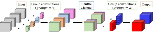
It is generally known that a regular convolutional kernel has spatial extent and channel extent, where the former value is always much smaller than the latter, for instance, a kernel with a size of “3×3×32×32”. Therefore, “group con-volutions” is proposed to remove the redundancy from the channel extent. It equally divides the input channels and the convolutional filters into several groups, and in every group , it performs the corresponding filters. “Group convolutions” can effectively reduce parameters and computations. How-ever, there are no interactions among the groups. This leads to the less accurate approximations of the regular kernel. To resolve this issue, the “shuffle channel” was proposed in ShuffleNet (Zhang et al. 2017).

Shuffle channel operation

(2)

Figure 1: General combinational structure of “group convolutions” and “shuffle channel” operations.

Motivation of super sparse convolutional kernel

Considering these issues, a new viewpoint is put forward in this paper for the first time that the feature maps’ general geometric characteristics and the information’s differentia-tion from different channels can be preserved through the selection of one pixel from every channel at different spa-tial locations. Accordingly, the introduced super sparse con-volutional (SSC) kernel in this paper should select the pix-els from the feature maps and perform operations on them by satisfying the above requirements. Consequently, a2 di-mensional spatial convolutional kernel is used to dilute and place its parameters into3 dimensions at the same spatial positions, which is called super sparse convolutional kernel. Figure 2 illustrates the comparisons of the regular convolu-tional kernel and the SSC kernel. It is notable that in this 3 dimensional kernel, every spatial kernel just has one pa-rameter. The SSC operations can be easily and more effi-ciently implemented by “shift”(proposed in Shift-Nets (Wu et al. 2017)) and “grouped point-wise” convolutional oper-ations without any spatial kernels (e.g., “3×3”). Shift-Net only removes the spatial’s redundancy, and group-conv mo-bile CNNs only removes the channel’s redundancy. How-ever, our SSC is the first method to remove the redundancy from both the spatial and channel extents at the same time. Furthermore, the SSC kernels can keep the spatial geomet-ric characteristic and maintain the channels’ differentiation based on its none-zero values’ locations. All of these factors lead to largely decreasing the model’s size than the other popular CNNs without performance loss and avoiding the over-fitting more effectively than the other state-of-the-art mobile CNNs.

Super sparse convolutional neural networks

Super sparse convolutional kernel

In Figure 2b, a SSC kernel can be seen as diluting a two dimensional spatial kernel (called the basic kernel) into a three dimensional kernel. In this way, the spatial non-zero locations are kept the same with thebasic kernel, which can preserve the general geometric characteristics. And the di-luting process can maintain the features’ differences along the channel extent. Suppose the4dimensional regular con-volutional kernel isT ∈Rk×k×C×D, wherek×kindicates

the spatial kernel size.CandDrefer to the number of input and output channels respectively. The SSC kernel is denoted byS ∈Rk×k×C×D. Then,S can be extended from the

ba-sic kernel W ∈ _Rk×k×D_{. It is noteworthy that in a SSC} kernel,C =k×k. Therefore, the definition of SSC can be

formulated as below:

Sx,y_i,j =

Wx,y_j , i=x×k+y

0, otherwise. (1)

Where x, y indicate the spatial location and x, y ∈ {0,1,2, ..., k−1}. Besides this,i∈ {0,1,2, ..., C−1}and j∈ {0,1,2, ..., D−1}.

Implementation of the SSC operations

Given an input tensorI ∈ Rw×h×C, which is conducted

by the novel SSC kernelT, and the relevant output tensor

O∈Rw×h×Dcan be obtained as following equation:

O(x, y, q) = C−1 X

p=0

k−1 X

i=0

k−1 X

j=0

T(i, j, p, q)

I(x+i−δ1, y+j−δ2, p).

(2)

Whereδ1 =δ2 =bk/2candq ∈ {0,1,2, ..., D−1}.

Ac-cording to the Equation 1, the computational process of the SSC operations can be simplified by the equation below:

O(x, y, q) = C−1

X

p=0

T(ip, jp, p, q)

I(x+ip−δ1, y+jp−δ2, p).

(3)

Where the (ip, jp)is the only one nonzero parameter’s spatial coordinate at thepthchannel andip×k+jp=p.

From Equation 3, it is clear that an output value at the specific spatial location can be computed through the sum-mation fromC times multiplication operations. Moreover, since every plane in a SSC kernel has one parameter, it can be transformed to a “point-wise” kernel. Furthermore, in or-der to preserve the spatial location relations in the comput-ing process, we use a shift kernel P ∈ Rk×k×C×D

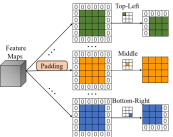
(in-troduced in (Wu et al. 2017)), which performs on feature maps to catch the features according to the SSC kernels’ non-zero spatial locations. The shift process operation is demonstrated in Figure 3. The definition of this shift kernel is shown as below:

Px,y_i,j =

1, Sx,y_i,j 6= 0

0, otherwise. (4)

Form Equation 3 and 4, the SSC operations can be further formulated as the following equation:

O(x, y, q) = C−1

X

p=0

T(p, q)P(ip, jp, p, q)

I(x+ip−δ1, y+jp−δ2, p).

(3)

(a) Regular convolutional kernel: the kernel hask×k×Cparameters (e.g., k= 3, C = 9), and it can be split toCspatial kernels along the channel extent.

(b) SSC kernel: the kernel hask×kparameters (e.g., k= 3), it consists ofC(C =k×k) spatial kernels, and every spatial kernel has only one non-zero parameter.

Figure 2: Comparisons of regular convolutional and SSC kernel.

Figure 3: Shift operational process: the feature maps are first padded with zero along each side, then each padded feature map is cropped based on the relevant shift kernel’s non-zero direction (the colored location in the shift kernel). In this figure, the shift kernel’s spatial size is “3×3” and the feature maps’ size is “4×4”.

From Equation 5, the SSC operation can be implemented by the “shift” and “point-wise” convolutional operations, which can save much more parameters and computational Flops.

The basic SSC module and the SSC-Nets

A “ point-wise” convolutional layer is first used to project the input feature maps into a required dimensional space, which can also fuse the previous module’s output features from different groups. The obtained projected feature map channels areM. Then, two SSC layers are equipped together with a “shuffle-channel” operation between them. Before each SSC operation, another “group point-wise” convolu-tional layer is utilized to force every SSC’s input to have similar geometric characteristics as much as possible. Fi-nally, similar to ResNets (Huang et al. 2016), identity map-ping is also adopted in the SSC module. The detailed struc-ture of a SSC-Net’s basic module is shown in Table 1.

It is important that in the second SSC layer, we still shift the feature maps and employ “point-wise” convolutional op-erations on everyC channels. Then, the number of groups

Table 1: SSC basic module. All the operations’ output chan-nels areM.C=k2andG=d×C.k2is the SSC kernel’s spatial size.

Stage Operation Groups Channels/Group

Conv1 1×1 1 M

Conv2 1×1 G C

1st_SSC shift G C

1×1 G C

Shuffle shuffle C G

Conv3 1×1 C G

2nd_SSC

shift G C

1×1 G C

1×1 C G

becomesG(G=d×C,dis a positive integer). Finally, an-other “group point-wise” convolution withCgroups is uti-lized to merge theGgroups toC groups. Hence, the SSC module entirely employs “wise” and “group point-wise” convolutions, which can largely decrease the param-eters and computational Flops. The SSC-Net uses the mod-ularized design method based on ResNet56 (Huang et al. 2016), SSC-Net also has three big blocks with different out-put spatial sizes (e.g.,32×32,16×16and8×8) and every block hasB basic modules. The output channels of every stage will be doubled when moving to the next stage. The other details remain the same with ResNet56(Huang et al. 2016).

Analysis of SSC kernels’ parameters

For a ResNet’s basic module in ResNet56 (Huang et al. 2016), suppose the kernel’s spatial size is “k×k” and the input and output channels areK. Therefore, a ResNet’s ba-sic module’s parametersPRare:

PR= 2×(k×k×K×K) = 2k2K2 (6)

(4)

SSC operation areG. Each group hasCchannels. Thus, the number of parametersPS of a SSC-Net’s basic module is:

PS=(1×1×M×M) + 2×(1×1×M×M/G)

+ 2×(1×1×M×M/C) + (1×1×M×M/G) =M2+ 3M C+ 2M2/C= (1 + 2/C)M2+ 3M C

(7)

From Equation 6 and 7, whenM =KandC=k×k,

PS =1

2

C+ 2

C2 +

3 M

PR≈ 1

2CPR. (8)

Therefore, whenkis3,C =k×k = 9andPS ≈ 1 18PR, which implies the SSC-Nets have much fewer parameters than the regular networks of the same width.

From another aspect, when the two modules have the same number of parameters (PS =PR),

K=

s

M 2

_C_{+ 2}

C2 M+ 3

≤1 2

_M

2 +

C+ 2

C2 M + 3

≈ ₁ 4 + 1 2C

M _≈ 1

4M,

(9)

this indicates SSC-Net is at least4Xwider than the regular model with the same parameters. Hence, SSC-Net can pro-cess and produce much more features. In addition, since the number of Flops is “w×h” (indicating the width and height of the feature map) times of the parameters, the SSC-Nets also have notable advantages when comparing the Flops.

Experimental result and analysis

Datasets

This paper’s goal is to design mobile models to reduce the number of parameters and computational complexity with-out any loss in performance and overcome the over-fitting problem on the less abundant datasets. As illustrated in (Chrabaszcz, Loshchilov, and Hutter 2017), since the low resolution ImageNet datasets’ spatial informations are much less abundant than the original ImageNet datasets, the low resolution ImageNet can make the model easily over-fitting and become more challenging than the original ImageNet. Therefore, we select the benchmark low resolution Ima-geNet and CIFAR (Krizhevsky and Hinton 2009) datasets.

CIFAR datasets (Krizhevsky and Hinton 2009) have a small number of images including CIFAR-10and CIFAR-100. They both have 60,000 colored nature scene images in total and the images’ size is32×32. There are50,000 images for training and 10,000 images for testing in 10 and 100 classes. Data augmentation is the same with the common practice in (He et al. 2016a; Huang et al. 2016; Larsson, Maire, and Shakhnarovich 2016).

Low resolution ImageNet datasets (Chrabaszcz, Loshchilov, and Hutter 2017) are the down-sampled vari-ants of ImageNet (Deng et al. 2009) and contain the same number of classes and images of ImageNet. There are three versions in total: ImageNet-64 ×64, ImageNet-32× 32

and ImageNet-16×16, which indicates the down-sampled images’ sizes are respectively 64 × 64, 32 × 32 and 16×16. In order to keep the same spatial size with CIFAR datasets, we perform SSC-Nets on ImageNet-32×32. The augmentation of this dataset is the same with (Chrabaszcz, Loshchilov, and Hutter 2017).

Initialization and hyper-parameters

The different versions of SSC-Nets, ResNet and Shift-Nets are respectively indicated by SSC-Nets-B-G, ResNets-B-ε and Shift-Nets-B-ε, whereBrepresents the number of basic modules in a big block.Gdenotes the number of groups in the first block.εis the expansion parameter (Wu et al. 2017). ResNets and Shit-Nets will have different model sizes by togglingε.

The almost identical weight initialization and optimiza-tion configuraoptimiza-tion introduced in ResNet are adopted in SSC-Nets. The mini-batch size is set to128. The SGD method and Nesterov momentum (Sutskever et al. 2013) are utilized in the optimization. Where the momentum is0.9. On CIFAR, the training epoch is set to160, and the optimization starts from the initial learning rate with0.1, which is divided by 10at the80th_and₁₂₀th_{epoch. For ImageNet, the training} epoch is40. The learning rate starts from0.01and is divided by10every 10 epoches. Finally, the weight decay is set to 0.0002and0.0001on CIFAR and ImageNet, respectively.

Parameter comparisons with approximately the

same accuracy

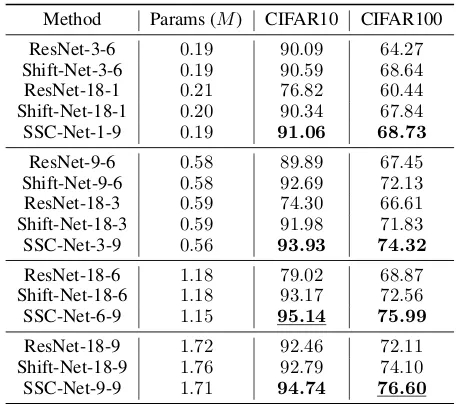
SSC-Nets and Shift-Nets both employ “point-wise” convo-lutions entirely, where SSC-Nets are implemented based on ResNet. Consequently, SSC-Nets are compared with Shift-Nets and ResShift-Nets. We first compare the models’ sizes under the approximately the same accuracy. The final number of parameters is shown in Table 2. The results of ResNets and Shift-Nets are reported in (Wu et al. 2017), and the value in the “params” column indicates a rough level of these two models’ parameters, since some models’ parameters and de-tailed structures are not illustrated in (Wu et al. 2017). It is apparent that SSC-Nets have much fewer parameters than the ResNets and Shift-Nets. SSC-Nets-2-9 reduces about

3.5Xparameters compared with ResNet-18-6 and Shift-Net-18-6. In addition, SSC-Net-3-9 also reduces about3.1X pa-rameters compared with ResNet-18-9 and Shift-Net-18-9. What is more, the results show that SSC-Nets can even achieve better performances than the compared models. For instance, SSC-Net-3-9 with0.56Mparameters improves the CIFAR10 accuracy by1.14%than Shift-Net-18-9. Addition-ally, compared with the best CIFAR10 accuracy 93.17% achieved by the Shift-Net-18-6 with 1.18M parameters, Shift-Net-18-9 with 1.76M parameters decreases the ac-curacy, which is caused by the over-fitting problem. How-ever, the larger model sized SSC-Nets-3-9 still outperforms SSC-Nets-2-9 through increasing the CIFAR10 accuracy by 0.69%. The experimental results show that the SSC-Nets can avoid this problem effectively.

(5)

Table 2: Comparisons of parameters with approximately the same accuracy (%) on CIFAR.

Method Params (M) CIFAR10 CIFAR100

ResNet-18-6 1.18 79.02 68.87

Shift-Net-18-6 1.18 93.17 72.56

SSC-Net-2-9 0.34 93.24 72.62

ResNet-18-9 1.72 92.46 72.11

Shift-Net-18-9 1.76 92.79 74.10

SSC-Net-3-9 0.56 93.93 74.32

Table 3: Accuracy (%) of SSC-Nets with1.5Xfewer param-eters compared with ResNets and Shit-Nets on CIFAR.

ResNet-9-6 0.58 89.89 67.45

Shift-Net-9-6 0.58 92.69 72.13

SSC-Net-2-9 0.34 93.24 72.62

ResNet-9-9 0.85 92.01 69.27

Shift-Net-9-9 0.87 92.74 73.64

SSC-Net-3-9 0.56 93.93 74.32

ResNet-18-9 1.72 92.46 72.11

Shift-Net-18-9 1.76 92.79 74.10

SSC-Net-6-9 1.15 95.14 75.99

consistently outperform ResNets and Shift-Nets. Compared with the largest ResNet and Shift-Net models, SSC-Net-6-9 achieves much better accuracies of95.14%and75.99%on CIFAR10 and CIFAR100 with only1.15M parameters.

Finally, the comparisons of parameters using Top-1 ac-curacy are performed on ImageNet-32×32 listed in Ta-ble 4. The experimental results show that SSC-Nets achieve a slightly better performance by utilizing2Xor2.5Xfewer parameters than ResNets. It proves that SSC-Nets can also perform effectively when facing more challenging datasets.

Accuracy comparisons with approximately the

same number of parameters

In order to test the performance when the model size of SSC-Nets increases, the accuracy comparisons are made by de-signing different SSC-Nets, whose parameters are approxi-mately the same with the relevant ResNet and Shift-Net. The final experimental results are shown in Table 5. It is notable that all SSC-Nets outperform the compared networks at their corresponding sized level. Especially, the the accuracies ob-tained by SSC-Net-3-9, where it increases by 1.24% and 2.19% on CIFAR10 and CIFAR100 compared with Shift-Net-9-6. The accuracies obtained by SSC-Net-6-9 increase by1.97%and3.43%on CIFAR10 and CIFAR100 compared with Shift-Net-18-6. Finally, compared with Shift-Net-18-9, the largest model SSC-Net-9-9 improves the CIFAR10 and CIFAR100 accuracies by1.95%and2.50%, respectively.

Additionally, on ImageNet-32×32datasets (see Table 6),

Table 4: Parameter comparison with approximately the same Top-1 accuracy (%) on Imagenet-32×32.

Method Params (M) Top-1 Reduction

ResNet-4-4 1.6 43.08

SSC-Net-3-9 0.8 43.88 2X

ResNet-4-8 3.5 48.94

SSC-Net-6-9 1.4 49.23 2.5X

Table 5: Accuracy (%) on CIFAR datasets with approxi-mately the same number of parameters.

ResNet-3-6 0.19 90.09 64.27

Shift-Net-3-6 0.19 90.59 68.64

ResNet-18-1 0.21 76.82 60.44

Shift-Net-18-1 0.20 90.34 67.84

SSC-Net-1-9 0.19 91.06 68.73

ResNet-9-6 0.58 89.89 67.45

Shift-Net-9-6 0.58 92.69 72.13

ResNet-18-3 0.59 74.30 66.61

Shift-Net-18-3 0.59 91.98 71.83

SSC-Net-3-9 0.56 93.93 74.32

ResNet-18-6 1.18 79.02 68.87

Shift-Net-18-6 1.18 93.17 72.56

SSC-Net-6-9 1.15 95.14 75.99

ResNet-18-9 1.72 92.46 72.11

Shift-Net-18-9 1.76 92.79 74.10

SSC-Net-9-9 1.71 94.74 76.60

Table 6: Accuracy (%) on ImageNet-32×32with approxi-mately the same number of parameters.

Method Params (M) Top-1 Top-5

ResNet-4-2 1.0 39.55 65.16

Shift-Net-4-2 1.0 41.47 67.44

SSC-Net-4-9 1.0 45.91 70.93

ResNet-4-4 1.6 43.08 69.08

Shift-Net-4-4 1.5 44.43 70.03

SSC-Net-6-9 1.4 49.23 73.81

ResNet-4-8 3.5 48.94 73.92

Shift-Net-4-8 3.5 51.85 75.88

SSC-Net-4-18 3.5 53.46 77.25

(6)

(a) CIFAR10acc (b) CIFAR100acc

Figure 4: Accuracy vs. parameters tradeoff.

(a) CIFAR10acc (b) CIFAR100acc

Figure 5: Accuracy vs. Flops tradeoff.

Comparisons with state-of-the-art mobile CNNs

Finally, in order to sufficiently explore the SSC-Nets’ per-formances, various SSC-Nets are compared with the other state-of-the-art mobile models. On the ImgeNet-32×32, Table.7 shows that SSC-Net achieves the best Top-1 and Top-5 accuracy than the other mobile models. It also proves that reducing spatial redundancy (SSC-Net and Shift-Net) can avoid over-fitting better than reducing channel redun-dancy (IGCV3-D 1.0), and SSC performs best because it re-ducing both the spatial and channel redundancy. Hence, the SSC-Net can remove the redundancy more thoroughly than the other mobile CNNs. On the CIFAR, from the Table. 8, it shows that the DenseNet is a optimal structure, because it uses the dense connections and bottle-neck to decrease the number of parameters and improve the performance. But, DenseNets are not very practical to be deployed on the mo-bile devices compared with the other group-conv momo-bile models, since the dense connections bring large memory storage in practice. For our SSC-Nets, it is clear that they can produce much better performances than the other group-conv mobile networks on CIFAR-10. As for the slightly dif-ficult CIFAR 100, since SSC is entirely implemented by the point-wise convolutions in practice, SSC-Net doesn’t achieve the best accuracy, but, it can also meet the general accuracy requirement.

Further investigation of the SSC kernel

The sparse property of the SSC Kernel In order to in-tuitively observe the sparsity of the SSC kernel. Accord-ing to (Ioannou et al. 2017), the filters’ relationships from two layers can be obtained through calculating the inter-covariances of the two successive layers’ response output channels. The corresponding inter-covariances from

differ-Table 7: Comparisons of accuracy (%) with the latest state-of-the-art mobile models on Imagenet-32×32.

Method Params (M) Top-1 Top-5

ResNet-4-8 3.5 48.94 73.92

MobileNetV2 3.5 48.98 73.82

IGCV-D1.0× 3.5 49.40 74.04

Shift-Net-4-8 3.5 51.85 75.88

SSC-Net-4-18 3.5 53.46 77.25

Table 8: Accuracy (%) comparisons to other state-of-the-art small and medium sized architectures on CIFAR.

Method Params (M)CIFAR10CIFAR100

Swapout (Singh, Hoiem, and Forsyth 2016) 1.1 93.42 74.14

DenseNet (Huang et al. 2017b) 1.0 94.76 75.58

DenseNet-BC (k= 12) (Huang et al. 2017b) 0.8 95.49 77.73

ResNet (Huang et al. 2017a) 1.7 94.48 71.98

ResNet(pre-act) (He et al. 2016b) 1.7 94.54 75.67

DFM-MP1 (Zhao et al. 2016) 1.7 95.06 75.54

MobileNetV2 (Sun et al. 2018) 2.3 94.56 77.09

IGCV2∗_-_C₄₁₆ _{(Xie et al. 2018)} ₀_.₇ ₉₄_.₅₁ ₇₇_.₀₅

IGCV2 (Sun et al. 2018) 2.3 94.76 77.45

IGCV3-D0.7× (Sun et al. 2018) 1.2 94.92 77.83

IGCV3-D1.0× (Sun et al. 2018) 2.4 94.96 77.95

Shift-Net-18-6 1.2 93.17 72.56

SSC-Net-6-9 1.2 95.14 75.99

SSC-Net-3-18 2.1 94.55 77.13

SSC-Net-4-18 2.8 94.95 77.67

ent stages of the Shift-Net and SSC filters are shown in Figure 6. The smaller the covariance, the sparser the filters are. From the Figure 6d, 6e and 6f, the SSC filters obtain an evident block diagonal sparsity, which implies the4 di-mensional SSC kernel is very sparse. Furthermore, in every group, all the3 dimensional SSC filters from the two suc-cessive layers are clearly clustered in a block with strong relationships, which effectively demonstrates that each 3 dimensional SSC filter can retrieve the specific geometric characteristics in its corresponding group. Consequently, the SSC kernel is more targeted and can process more informa-tion efficiently. This contributes to obtaining better features through its super sparse structures and effectively preventing any over-fitting.

(7)

re-(a) Stage1of Shift-Nets (b) Stage2of Shift-Nets (c) Stage3of Shift-Nets

(d) Stage1of SSC-Nets (e) Stage2of SSC-Nets (f) Stage3of SSC-Nets

Figure 6: Inter covariances of SSC-Nets and Shift-Nets.

(a) On0.19M params (b) On0.87M params (c) On1.76Mparams (d) Various SSC-Nets

Figure 7: Comparisons of sparsity ability on CIFAR10.

veals the real nature of SSC’s sparsity ability and the rea-son why sparse models can avoid over-fitting better on the less abundant dataset. Additionally, when the model size be-comes larger, Shift-Net’s sparsity ability decreases gradually until almost to same extent with ResNet. However, from Fig-ure 7d, when the model size increases, SSC-Net’s sparsity ability is also improved. This proves that SSC can combat over-fitting more effectively on the less abundant datasets.

Conclusion

A novel super sparse convolutional kernel (SSC) is proposed in this paper. The SSC kernel is much sparser than the tra-ditional convolutional kernel, since it is the first method to reduce the parameters’ redundancy from both the spatial and the channel extents at the same time. Additionally, the re-trieved features by the SSC kerenl can preserve the gen-eral characteristics of the geometric and the channels’

dif-ferences and the computational Flops can be also largely decreased. Finally, it is effectively implemented by “shift” and “group point-wise” convolutional operations. Experi-mental results show that SSC-Nets can effectively decrease the model’s size without any performance losses and address the over-fitting better than the other state-of-the-art mobile networks on the more challenging less abundant databases.

Acknowledgments

This work is supported by NSFC fund

(61332011), Shenzhen Fundamental Research fund

(8)

References

Chrabaszcz, P.; Loshchilov, I.; and Hutter, F. 2017. A down-sampled variant of imagenet as an alternative to the cifar datasets.arXiv preprint arXiv:1707.08819.

Deng, J.; Dong, W.; Socher, R.; Li, L.-J.; Li, K.; and Fei-Fei, L. 2009. Imagenet: A large-scale hierarchical im-age database. InComputer Vision and Pattern Recognition, 2009. CVPR 2009. IEEE Conference on, 248–255. IEEE. Dong, X.; Chen, S.; and Pan, S. 2017. Learning to prune deep neural networks via layer-wise optimal brain surgeon. In Advances in Neural Information Processing Systems, 4860–4874.

Han, S.; Pool, J.; Tran, J.; and Dally, W. 2015. Learning both weights and connections for efficient neural network. In

Advances in Neural Information Processing Systems, 1135– 1143.

He, K.; Zhang, X.; Ren, S.; and Sun, J. 2016a. Deep residual learning for image recognition. In The IEEE Conference on Computer Vision and Pattern Recognition (CVPR), 770– 778.

He, K.; Zhang, X.; Ren, S.; and Sun, J. 2016b. Identity mappings in deep residual networks. InEuropean Confer-ence on Computer Vision, 630–645. Springer International Publishing.

Howard, A. G.; Zhu, M.; Chen, B.; Kalenichenko, D.; Wang, W.; Weyand, T.; Andreetto, M.; and Adam, H. 2017. Mo-bilenets: Efficient convolutional neural networks for mobile vision applications. CoRRabs/1704.04861.

Huang, G.; Sun, Y.; Liu, Z.; Sedra, D.; and Weinberger, K. 2016. Deep networks with stochastic depth. InEuropean Conference on Computer Vision, 646–661. Springer Inter-national Publishing.

Huang, G.; Li, Y.; Pleiss, G.; Liu, Z.; Hopcroft, J. E.; and Weinberger, K. Q. 2017a. Snapshot ensembles: Train 1, get m for free. arXiv preprint arXiv:1704.00109.

Huang, G.; Liu, Z.; Weinberger, K. Q.; and van der Maaten, L. 2017b. Densely connected convolutional networks.arXiv preprint arXiv:1608.06993v4.

Hubara, I.; Courbariaux, M.; Soudry, D.; El-Yaniv, R.; and Bengio, Y. 2016. Binarized neural networks. InAdvances in neural information processing systems, 4107–4115. Ioannou, Y.; Robertson, D.; Cipolla, R.; Criminisi, A.; et al. 2017. Deep roots: Improving cnn efficiency with hierarchi-cal filter groups.

Krizhevsky, A., and Hinton, G. 2009. Learning multiple layers of features from tiny images.

Larsson, G.; Maire, M.; and Shakhnarovich, G. 2016. Frac-talnet: Ultra-deep neural networks without residuals. arXiv preprint arXiv:1605.07648.

Lin, J.; Rao, Y.; Lu, J.; and Zhou, J. 2017. Runtime neu-ral pruning. InAdvances in Neural Information Processing Systems, 2178–2188.

Lin, X.; Zhao, C.; and Pan, W. 2017. Towards accurate binary convolutional neural network. InAdvances in Neural Information Processing Systems, 344–352.

Sandler, M.; Howard, A. G.; Zhu, M.; Zhmoginov, A.; and Chen, L. 2018. Inverted residuals and linear bottlenecks: Mobile networks for classification, detection and segmenta-tion. CoRRabs/1801.04381.

Singh, S.; Hoiem, D.; and Forsyth, D. 2016. Swapout: Learning an ensemble of deep architectures. In Advances in neural information processing systems, 28–36.

Sun, K.; Li, M.; Liu, D.; and Wang, J. 2018. Igcv3: Inter-leaved low-rank group convolutions for efficient deep neural networks. CoRRabs/1806.00178.

Sutskever, I.; Martens, J.; Dahl, G.; and Hinton, G. 2013. On the importance of initialization and momentum in deep learning. InInternational conference on machine learning, 1139–1147.

Wu, B.; Wan, A.; Yue, X.; Jin, P.; Zhao, S.; Golmant, N.; Gholaminejad, A.; Gonzalez, J.; and Keutzer, K. 2017. Shift: A zero flop, zero parameter alternative to spatial con-volutions. arXiv preprint arXiv:1711.08141.

Wu, J.; Li, D.; Yang, Y.; Bajaj, C.; and Ji, X. 2018. Dynamic sampling convolutional neural networks. arXiv preprint arXiv:1803.07624.

Xie, G.; Wang, J.; Zhang, T.; Lai, J.; Hong, R.; and Qi, G. 2018. IGCV2: interleaved structured sparse convolutional neural networks. CoRRabs/1804.06202.

Zhang, X.; Zhou, X.; Lin, M.; and Sun, J. 2017. Shufflenet: An extremely efficient convolutional neural network for mo-bile devices. arXiv preprint arXiv:1707.01083.