Water supply reliability theory

Full text

(1)Water supply Uri Shamir and Charles. reliability. theory. D.D. Howard. Water supply system reliability can be defined in terms of the shortages that result from failures of a system’s physical components. A reliability factor for a single failure or for a selected time period can be defined in terms of the capacity lost during failure, which is measured as a fraction of the demand rate or the demand volume. Since the lost capacity is a random variable, so is the reliability factor, and its probability density function can be derived analytically from that of the lost capacity. Reliability, defined as the probability that a given reliability factor will be achieved, can be increased by adding facilities, storage, pumping capacity, pipelines. The least-cost combination of facilities can be identified from the cost functions and the probability distributions of the reliability factor. In 1972, Damelin, Shamir, and Arad’ outlined the considerations involved in assessing water supply reliability. They developed a computer simulation model that was used to evaluate reliability for specific water and supply systems defined a reliability factor in terms of shortages in annual delivery volumes. Because the system is subject to random failures of pumping equipment and of electrical power supply, the reliability factor is a random variable. Analysis of its random nature was performed through repeated runs of the stochastic simulation. An economic model was based on this analysis. Mathematical functions developed by the authors are used to describe reliability and to develop a framework for its economic assessment. The new procedure is a screening model that provides preliminary solutions based on an approximate, analytical, optimization model. These solutions can be used as a basis for a more complete analysis by simulation. The effect of a supply failure on a system’s reliability depends on system demand at the time the failure occurs. The analysis in this paper is based on the demand being fixed and known. Real system demand varies over time and has JULY. 1981. a random component. Therefore, the reliability analysis developed herein addresses only one part of the overall prohlem. Future work will deal with the random nature of both demand and supply. Definition of a reliability factor A natural way to define water supply. system reliability is in terms of the shortfalls relative to the desired demand. Demand for water may he considered in terms of the rate of supply required, in units of discharge, or in terms of the total volume to he supplied over a given period of time. Other considerations may relate to the number of failures per time, regardless of the length or magnitude of each, and to the total duration of the failures during a time period, e.g., one year. The authors define reliability in terms of total volume and supply rate shortfalls. Together these factors suggest the possibility that a short-term loss of the entire supply may have a more serious effect than a longer-term loss of only a portion of the capacity, even if the volume of the shortfall is the same in both cases. The overall reliability can be considered to depend on two components. The first is the discharge reliability factor, RC. (1) where C is the capacity rate in units of discharge, lost because of the failure, out of the total rate required CT. Values of the power n greater than 1 cause RC to decrease very rapidly as C approaches CT. Values of n less than 1 cause RC to drop rapidly for small values of the shortfall C (Figure 1). The second component is the volume reliability factor, RV. 0. 05. I[. Relative Shorlfall--C,CT. Figure. 1.. Reliability. 0003-150X/81 0 1981 American. factor shortfall. versus. /070379-06$02.00 Water. Works. Copyright © 1981 American Water Works Association. Assoaat~on. relative. where V is the shortfall volume during a single failure or during an entire time period (e.g., one year) out of the total volume desired VT. V is a product of the lost capacity rate C and the length of U. SHAMlR. & C.D.D.. HOWARD. 379.

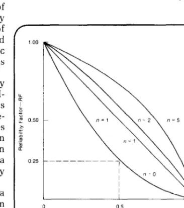
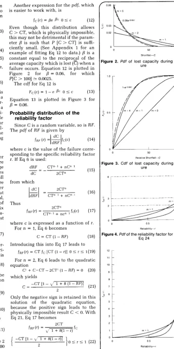
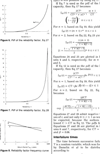
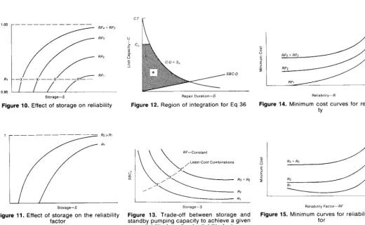
(2) time required for repair and restoration of full supply D. By using these two factors, the overall reliability factor can be defined as follows: RC + RV RF = ~. (3). 2. For a single failure event V= C-D. (4). VT = CT-D. (5). in which D is the duration of the failure, the reliability factor can be written. RF = 1 _ (C/CT)” + (C/CT) 2. (6). The reliability theory is based on this definition. Alternative definitions of a reliability factor could include consideration of the total number of failures in a given time period, the duration of periods without failures, and the magnitude or duration of the worst failures.’ For each alternative definition of the reliability factor it is possible to develop the alternative reliability theory, following the procedure described herein.. Shortfall. probability. There are many components in a water supply and distribution system that are subject to failure. Water main breakage is a common source of failure that causes a relatively small reduction in the overall delivery capability of the system. Failure of a major supply aqueduct or a water treatment plant may be infrequent, but the result is a substantial, or even total, loss of capacity. Based on an analysis of the data in Damelin et al (see Appendix l), the authors postulated that the probability density function (pdj) for lost capacity is of the general form. fc(d = =&-&)“‘O”cSCT. fc (c) = ,8e PC 0 5 c. oic<CT. (8). (12). Even though this distribution allows C > CT, which is physically impossible, this may not be detrimental if the parameter ,!? is such that P [C > CT] is sufficiently small. (See Appendix 1 for an example of fitting Eq 12 to data.) ,B is a constant equal to the reciprocal of the average capacity which is lost (c) when a failure occurs. Equation 12 is plotted in Figure 2 for p = 0.06, for which P[C > 1001 N 0.0025. The cdf for Eq 12 is F&)=1-eb. OSc. Equation 13 is plotted p = 0.06.. g 05 c. (14). =l$jfCic). CT”-’. --. dC-. correfactor. (15). 2CT”. Probability [-& 5 a] = p. (9). If Eq 8 is used, this results in 1 - (1 - c-p-1 = p. (10). from which the value of m is given by Ill=. 1% Cl- P) _ 1 log (1 - a). 380. RESEARCH AND TECHNOLOGY. 0. 50. 100. ‘igure 3. Cdf of lost capacity ure. during. a fail-. from which. I I. 2CT”. dC PC dRF. Thus fRF(d. =. CT” 1 + nC”-’. (1’3). zCT” CT”-’ + nc” l fdc). (17). where c is expressed as a function For n = 1, Eq 6 becomes C = CT(l-RF) Introducing. of r.. (18). :igure 4. Pdf of the reliability factor for n = 1, Eq 24. this into Eq 17 leads to r)] 0 % r 5 l(19). fRF(r) = CT fc [CT (I-. For n = 2, Eq 6 leads to the quadratic equation (20). which yields. c-. c = -CT [l - J ‘, + 8 (1 - RF)]. (21). Only the negative sign is retained in this solution of the quadratic equation, because the positive sign leads to the physically impossible result C < 0. With Eq 21, Eq 17 becomes 2CT fRF(‘). (11). The pdf from Eq 7 is plotted in Figure 2 for CT = 100 (e.g., a total capacity of 100 ml/h) and for m = ~2, and 5. The cdf from Eq 8 is plotted in Figure 3 for m = 1,2, and 5.. 0 Relatwe Shortfall-c. + nC” 1. CJ + C * CT - 2CT’ (1 - RF) = o. The parameter m can, for example, be computed from recorded information that gives:. a fail-. so is RF.. where c is the value of the failure sponding to the specific reliability r. If Eq 6 is used: dRF. during. 3 for. of the. Since C is a random variable, The pdf of RF is given by fRF (d. :igure 2. Pdf of lost capacity ure. (13). in Figure. Probability distribution reliability factor. (7). with m > 1 a parameter to be determined from data. The cumulative distribution function (cdj) for lost capacity is F&c)=l-(1-&)m-l. Another expression for the pdf, which is easier to work with, is. -CT. =. J. 1. +. 8(1. [l - ,/ 1 + a(1 - r)] 2. -. r). fc. 0 5 r I1. (22). For other values of n it may not be possible to express C = C(RF) explicitly from Eq 6; a numerical evaluation of. 1 m=1 00[l&d&!‘! 05 10 Rellablllty-r Figure 5. Pdf of the reliability factor for n = 2, Eq 25. Copyright © 1981 American Water Works Association. JOURNAL AWWA.

(3) far(r) is still possible by using Eq 17. If Eq 7 is used as the pdf of the lost capacity, then Eq 17 becomes ZCT" fHF@). J. =. Repair duration. CT. ’. (23). fH,c (r) = (m + 1) rm 0 I r I. 1. (24). For n = 2, based on Eq 22, Eq 23 yields 2 (m + 1). Figure 6. Pdf of the reliability factor, Eq 27 fRF@). =. J. 1 + 8(1 - r). 1 1 + 8(1 - r) 1” 0 5 r I 1 (25). [l+1-v. 2. Equations 24 and 25 are plotted in Figures 4 and 5, respectively, for m = I,& and 5. If Eq 12 is used as the pdf of the lost capacity, then Eq 17 becomes 2CT” fw(4. =. CT”. 1 +. nC,,mlBe. Mr). r 5. 1(26). For n = 1, based on Eq 19, this yields fRF tr) = CT - /3emb[cT(l - 41 r 5 1 (27) For n = 2, based becomes. on. Eq. 22, Eq. 26. 2PCT fRF (r). 0 0. I 100. I ,000. Ret”,” Period r,,o--years. Figure 8. Reliability factor frequency. curve. =. \/ 1 + 8(1 - r). exp BCTll- v’ ’ + ‘(’ I 2. - ‘)I} r 5 1 (28). times. The time between successive failures T is a random variable, which was found by Damelin et al to be distributed according to fT (t) = X e-At t 2 0. Return period of the reliability factor. JULY 1981. for Eq 33. Damelin et al found that repair duration D is well described by the lognormal distribution.. fdm) = \lzn. (29). X = l/T is the reciprocal of the mean time between failures (MTBF) and is therefore the average number of failures per time unit. If T is measured in years, then X is the average number of failures per year. The statistical parameter h is related to maintenance; as maintenance improves, h should decrease.. Figure 9. Region of integration. (30). Interfailure. nC". For n = 1, based on Eq 19, this yields. I 10. XP[RF i RFo] = XF,F (RF,). the. Equations 27 and 28 admit negative values of r, and not only 0 I r i 1 as would be expected, because the authors allowed C > CT in Eq 12. The pdfs from Equations 27 and 28 are plotted in Figures 6 and 7, respectively, for CT = 100 and p = 0.06.. I+. O<r%l. I 1. ‘TRF, =. m+l. .-.. quantities,. This result defines a reliability factor frequency curve that can be used in comparing the reliability of alternative systems. For example, Figure 8 shows this relationship for two hypothetical alternatives, A and B. They have the same reliability factor at a return period of 10 years, but differ considerably at other return periods. In this instance, alternative B is normally more reliable (at return periods of less than 10 years) but on rare occasions becomes much less reliable than alternative A, which has a more stable behavior. Choice of the best alternative depends on the relative benefits and damages that result from more frequent, relatively small shortfalls and from rarer but larger ones. The factors of interest in comparing the reliabilities of alternative systems may be the slope of the frequency curve and the reliability factor at some conveniently defined return period. The return period shown in Figure 8 indicates the average number of years between times when the reliability factor fails below the designated level. It is also useful to estimate the probability that the reliability factor will not fall below the designated value during a certain number of years. This can be accomplished by assuming a reliability factor RF, with an average return period of = 10 years. If successive shortfalls T ar?statistically independent, then the probability of not experiencing a shortfall with RF < RF, over a lo-year period is approximately 0.33 (computed from a binomial distribution).. CT". 3. Figure 7. Pdf of the reliability factor, Eq 28. calculated. Using annual return period is. The associated reliability factor can be computed for each shortfall. The same can be done for any selected time period. If a reference value of the reliability factor RF,, is selected, the average length of time it takes before the reliability factor drops below this value can be. exp. 1. M. - ,&I&-. (31) o<*. BM. I. where m = log (repair duration, I)). &? and ohl are the mean and standard deviation, respectively, of the logarithms of the repair durations. For sufficiently large values of the repair durations, a different pdf can be used for the repair duration to make further computations easier. f,,(d) = e ‘I’ d 0 5 d (32). Variation. of demand. In the preceding discussion, demand was assumed to be constant. Real demand for water changes over time and typically shows patterns of daily and U. SHAMIR & C.D.D. HOWARD. Copyright © 1981 American Water Works Association. 381.

(4) storage--S. Figure 10. Effect of storage on reliability. Figure 12. Region of integration. for Eq 36. Figure 14. Minimum cost curves for reliabilitY. >. t-. R2 w S’. Figure 11. Effect of storage on the reliability factor. Figure 13. Trade-off between storage and standby pumping capacity to achieve a given reliability for a fixed reliability factor. Figure 15. Minimum curves for reliability factor. seasonal variation. Demand also usually increases over the years. Moreover, there is a random component to demand, making it unpredictable except in a probabilistic sense. Demand is taken into consideration in the definition of reliability. Even if the supply capability has the same probability of failure at all times, the reliability factor will change as the demand probability changes. A complete analysis of reliability will, therefore, consider both supply and demand as random variables.. of storage in reliability of supply is an example. A practice commonly employed in the water industry can be used to illustrate how a probability factor can be determined. If a pump failure occurs at the source and that water can be supplied directly from a reservoir while this failure is being repaired, the storage volume S needed to cover the shortfall is a product of the lost capacity C and the time necessary to repair the failure D. The probability density function of the required storage can be derived from those of the failed capacity and the repair duration. This is illustrated schematically in Figure 9. The probability that a storage volume s,, will meet consumer demand during a failure event is. the absence of specific data, independence might be assumed. Equation 33 then becomes P[C . D 5 s,] = e fdd)dc fn(d)dd (34). Improving. supply reliability. Water supply reliability may be improved by means of a variety of measures, such as l Additional production capacity of sources, i.e., wells, pumping stations at surface sources, water treatment plants; l Standby pumping capacity at wells or pumping stations; l Additional storage; l Increased conveyance capacity of the transmission lines from the sources; 0 Additional pipelines in the distribution system; and l Improved maintenance of pumps, pipes, and other components. When a particular system is being studied, specific characteristics must be investigated. The evaluation of the role 382. RESEARCH AND TECHNOLOGY. P[C - D I s,,] = {if, “(cd). dc dd. (33). where D is the area in which (C * D 5 S,,), as indicated by the shaded area in Figure 9. If the storage reservoir has a volume S,, and if it is assumed that sufficient time is available between failures to replenish the reservoir, then Eq 33 gives the probability that no shortfall will occur during a failure. It is possible that lost capacity during a failure and the repair duration are not statistically independent. However, in. with the two pdfs given in previous sections. For failures with a capacity loss below value C,, P[C . D < S,,l a specified C < CO] can be computed by restricting the integration to that part of a below C = C,. For each value of C, the corresponding reliability factor RF, can be computed by using Eq 6 with the appropriate value of n. Thus R (RF,,S,) = P[RF I RF, 1S = S,] = P[C.D < S, 1 C < C,] (35) A schematic diagram of the results of this computation is shown in Figure 10. The probability R is called the reliability and serves in this example as a function of the reliability factor (a measure of the lost capacity) and the storage. When the probability functions f<;(c) and f,(d) are not given in analytical forms but as histograms or data tables, it is still possible to make the computations to evaluate the reliability curves directly from the data. For a selected reliability value, e.g., R,, it is possible to construct an isoreliability curve that will show the trade-off. Copyright © 1981 American Water Works Association. JOURNAL AWWA.

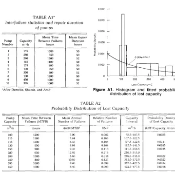
(5) TABLE Al’ statistics and repair durution af pumps. Interfailure. Pump Number. Mean Time Between Failures hours. Capacity w/h. Mean Rrpatr Duration hours. 1 2 3. 115 28” 280. 1300 65” 15””. 5” 5” 57.. 5 6 47. 153 13” 350 115. !a! “5” 8”” 1100. 5” 5” 52 .s”. ‘After. Damelin.. Shamir.. 0 008 c. z :. 0 002 1.. Figure Al. Histogram and fitted probability distribution of lost capacity. and Arad’. TABLE A2 Distribution of Lost Capacity. Probability Pump Capdcity. Mean Time Betwren Fadures (MTFB). Mean Annual Numbrr of Fdilurrr. m3/h. hours. 84OUIMTBF. 1”” 115 115 13” 153 280 28” 350 3% 45”. 12”” 11”” 13”” “5” ““0 65” 15”” 8”” l”“” loo”. 7.0” 7.64 6.46 8.84 0.33 12.92 5.6” 10.5” H.4” 8.4”. Relative Numbrr of Faduri:.s RNF U.062 O.166 0.166 0.104 0.11” 0 218 0.218 0 123 0 “99 0.099. Probahdtty DenQy uf Lust Capacity m3/h. RNFICdpdcity. intervdl. a.0055 0 “111 0 ““55 0.0015. 4x2.5-477.5. “.““ZZ 0.0022 0.0014 0.001”. time. The data required to perform the analysis should be readily available in the maintenance records of water supply agencies, since interfailure times and repair durations are the only data needed. If such data are available, they should be used to develop reliability factors and associated probabilities-the only way to determine which facilities, if any, should be expanded or added to the system to increase reliability. When a system must be expanded to meet rising demands, the plan for expansion should consider reliability as part of the criteria for assessing alternatives. A procedure can be developed to determine which alternative measures provide the desired reliability, so that the best alternatives can be identified. This procedure was demonstrated for the alternatives of additional storage versus standby pumping capacity. The same could be done for a trade-off between new aqueduct capacity and terminal storage or additional treatment capacity. The analysis presented here has not considered the reliability of the sources in terms of the hydrological behavior of the watershed or aquifer. It should be possible to extend this analysis to include such an assessment by replacing the failure probability density functions with functions that describe the natural availability of water at the sources.. Appendix 1 Probability density functions from data between the reliability factor RF and storage S (Figure 11). The right-hand scale in Figure 11 is expressed in terms of the relative lost capacity C/CT, a unique function of RF, obtained from Eq 6. (For n = 1 the scale transformation from RF to C/CT is linear; see Figure 1.) Assume that it is possible to install standby pumps at the source. These pumps would be placed in operation when repairs were being made to failed main pumps. The reliability factor can be increased by the addition of these standby pumps, by additional storage, or by combinations of these two measures. For any combination of lost capacity C,, reservoir volume S,,, and standby pump capacity SBC,, the reliability R can be computed by integrating the joint probability function fc,D(c,d) over the region 0 shown in Figure 12: R (RF,, S,,, SBCJ = Jlf(;(c)dc f,(d) dd (Q) Results are plotted in Figure selected value of the reliability. Economic. (36) 13 for a factor.. optimization. Isoreliability curves can be used in an economic optimization of a system. Consider, for example, the system discussed in the preceding section. For every isoreliability curve, it is possible to compute JULY 1981. the cost of the combinations of storage and standby pumping capacity and then determine the least-cost combination (Figure 13). These results can be plotted in two other ways: minimum cost versus R for a fixed value of RF (Figure 14) and minimum cost versus RF for a fixed value of R (Figure 15). Figures 14 and 15 show the expected outcome: as R approaches 1.0 for any value of RF, the cost curve becomes steeper. The marginal cost of reliability rises sharply as higher reliability is desired. These results can aid in selecting an appropriate level of reliability. If it is possible to pinpoint damages resulting from shortfalls, then costs and benefits can be balanced to yield the optimal system. More often, however, it is not possible to quantify these damages. The decision must then be based on an observation of cost curves (Figures 14 and 15) to locate a reasonable reliability value.. Conclusion Reliability computations for water supply systems depend on the definitions used. It is possible to develop a comprehensive statistical description of reliability by defining a reliability factor that is a function of the relative shortfall during a failure or over some period of. Damelin, Shamir, and Arad present some statistical data on interfailure times and repair duration. From this data it is possible to approximate the probability distribution of lost capacity. This is done by considering separately the interfailure statistics that are given for each pump, along with its capacity. These data (Table Al) were reorganized and analyzed as follows: 1. Pumps are arranged in ascending order of capacity. 2. It is assumed that all pumps operate 8400 hours per year. This is equivalent to 700 hours of work per month, with some 20-44 hours for preventive maintenance and other scheduled outages. 3. The relative number of failures of the specified pump capacity RNF is the mean annual number of failures of the particular pump divided by the total number of annual failures of all pumps. 4. The probability density of lost capacity is the relative number of annual failures RNF divided by the capacity interval which it represents. 5. Pumps of equal capacity are grouped by adding their RNFs. The total pumping capacity in the water supply system which is analyzed here is 2368 ml/h. The analysis is based on the assumption that the probability of two or more pumps failing simultaneous-. Copyright (C) 1981 American Water Works Association. U. SHAMIR & C.D.D. HOWARD. 383.

(6) -. ly is negligible. The results are given in Table A2 and plotted in Fig Al. A gamma or log-normal distribution could have been used to fit the data, but over the range of lost capacity that is of interest, say above 200 ml/h (about 10 percent of the total capacity), the exponential distribution (Eq 12) may be adequate. The parameter of the distribution may be fitted in several ways. One would be to make it equal to the reciprocal of the mean capacity which is lost, 245 ml/h, i.e., fl g 0.004. Another way would be to set the parameter so that the probability of exceeding some given value of the lost capacity is as found in the data. For the given data these also lead to a value of /? close to the one given above. The exponential distribution with fi = 0.004 is shown in Figure Al.. Calculating. Appendix 2 probabilities in Eq 35. If lost capacity C and repair duration D are independent and exponentially distributed, then the computation of the reliability in Eq 35 is performed as follows, based on Figure 9 and the area below the line C = C,: P[C * D < SJC < C,,] =. {‘o fc(c) dc. ;‘,,”. fo(d) dd. With Eq 12 and Eq 32 as the pdfs of C and D, respectively, the integration yields ‘0 e PCdc JS”/C e-9l dt ?/ 0. The last integral must be evaluated numerically, which can be done with a programmable calculator. The results are shown schematically in Figure 10.. References 1. DAMELIN, E.; SHAMIR, U.; & ARAD, N. Engineering and Economic Evaluation of the Reliability of Water Supply. Water Resources Res. 8:4 (Aug. 1972). 2. YEN, B.C. Safety Factor in Hydrologic and Hydraulic Engineering Design. Proc. Intl. Symp. Risk and Reliabilit: in Water. Uri Shamir is a professor of civil engineering at Technion in Haifa, Israel, and Charles D.D. Howard is president of Charles Howard & Associates, Ltd., 500-455 Granville St., Vancouver, BC V6C lV2.. Copyright (C) 1981 American Water Works Association 384. RESEARCH AND TECHNOLOGY. JOURNAL AWWA. ..

(7)

No results found