Chapter 5 Transient Conduction

C

HAPTER

5:

T

RANSIENT

C

ONDUCTION

In practical terms, very few processes operate at a true steady-state.

Variations in operation may arise from “noise” caused by controller accuracy and/or mechanical variation inherent to the different pieces of equipment that make up the process

! Processes such as this may be

considered to be at steady state

For other processes, disturbances consistently arise, causing the

controller to continuously adjust to search for the specified set-point

! Processes such as these virtually

always operate in transient mode. dT/dt ≠≠≠≠ 0

D

EALING

W

ITH

N

ON

-S

TEADY

S

TATE

C

ONDUCTION

Transient conduction may be simple or extremely difficult to consider,

depending on the assumptions applied. Consider the case of

suddenly changing the temperature of one surface of an object.

If temperature gradients within the

solid may be neglected (small, high k)

" lumped capacitance method

If the only significant temperature

gradient is 1D " approximations of

heat diffusion equation solutions

If significant temperature gradients exist in 2-3 dimensions " finite

element/finite difference method

L

UMPED

C

APACITANCE

M

ETHOD

The lumped capacitance method can be used to find dT/dt if it is assumed that the temperature T(x,y,z) is

identical throughout the entire object

at any instantaneous time point.

With no spatial variation in T, d2_T/dx2_,

d2_T/dy2_{, and d}2_T/dz2 _{are all zero.}

This assumption is reasonable when R(conduction through body) (∆x/kA)

<< R(heat loss at surface) (1/hA)

" if the body is very small

" if the thermal conductivity (k) is

very large (k " ∞)

" if h, hr are small

= +     

  

   

 

∂ ∂ +    

 

∂ ∂ +    

 

∂ ∂

q z

T y

T x

T

k ₂ &

2 2

2 2

2

t T c_p

∂ ∂

ρ

Common situation: an object initially at temperature T1 is immersed in a

cooling fluid at temperature T2

" the object loses heat by convection

from the surface to the surroundings

If no internal heat generation is taking place (q = 0), the energy balance is:

− E&out = −E&conv = E&st

(heat loss by convection = internal energy change)

(

)

dt dT V

c T

t T

hA_s − =

ρ

_p

− ( ) _∞

cp = heat capacity (per unit mass)

V = volume of solid body

Q: Why can’t we directly use the

general heat diffusion equation to do this balance?

Ti T(t)

T∞ < Ti

t < 0 t ≥ 0

.

We can solve this equation in the same manner as we did for fins. Let

θ

= T −T∞ , such that

(

)

V c T T hA dt dT P s

ρ

∞ − − =

"

_ρ

θ

θ

V c hA dt d P s − =

Separating variables,

∫

= −

∫

t p s dt V c hA d

i

θ

ρ

0

θ

θ

θ

No x, y, or z dependence on temperature " no boundary

conditions required to solve problem

Time dependence on temperature

(first derivative) " we need one initial

condition to solve this problem: @ t=0, T=Ti, or Ti-T∞ = θi

Integrating (LHS = ln(θ)-ln(θo) =

ln(θ/ θo) and taking exponentials:

      − = t V c hA P s o

ρ

θ

θ

exp

" _

Thermal Time Constant

Based on this result, we can define the thermal time constant τt as the

inverse of the pre-exponential factor which determines the rate of

exponential heat loss from the object:

(

p

)

t t s

t c V R C

hA _ =

 

 

=

ρ

τ

1

Thus, the higher the resistance to heat transfer Rt (via convection only

in this case) and the higher the

lumped thermal capacitance Ct of the

solid (capacity of the object to store heat), the longer it will take to reach the new steady-state condition

" parallel to electricity – more

capacitance = lower discharge rate 

  

 

− =

− −

∞ ∞

t i

t T

T

T T

τ

exp

Heat Flow From a Lumped Object

From the energy balance, all heat lost must be due to convective dissipation. i.e. ∆Eout = Q = -∆Est . Thus,

= =

∫

⋅ =

∫

⋅

t

s t

conv

t Q q dt hA dt

Q

0 0

θ

Q is the total heat transferred (J) q is the heat flow rate (J/s = W)

Integrating and applying the definition for θ from the previous equation,

Remember: q is positive if from surface, negative if to surface.

Thus, positive q ! negative Est

(reduction in temperature of object)

" this is what we would expect

(

)

_

  

 

   

 

− −

=

t i

P

t V

c Q

τ

θ

ρ

1 exp

E

VALUATING THE

V

ALIDITY

OF

L

UMPED

C

APACITANCE

While the attractiveness of using

lumped capacitance is clear from the simplicity of the resulting equations, we need a way to evaluate whether or not the assumptions we made in

deriving the equations are valid for a given system we are analyzing.

Key assumption: R(conduction through body) << R(heat loss at surface) [e.g. R (convection)]

To evaluate this, take the ratio of the conductive and convective resistance. For a plane wall (Ac=As) of thickness L

Biot Number

_Bi

k

hL

hA

kA

L

R

R

s c

conv

cond

=

=

≡

1

If the Biot number is low, Rcond<<Rconv

and assumptions used to derive the lumped capacitance model are valid

i.e. = = _dz = 0

dT dy

dT dx

dT

and k " ∞

The error associated with these

assumptions is sufficiently small when

Bi = hL_kc < 0.1

where Lc ≡ V/As for a given object

Lc should correspond to the length

scale with the maximum spatial temperature difference

i.e. for a “long” cylinder "

semi-infinite assumption is valid " virtually

all heat loss occurs radially such that Lc = r instead of (πr2L/2

π

r) = r/2 as

suggested by the general formula

G

ENERAL

L

UMPED

C

APACITANCE

M

ETHOD

Up to now, we have only considered heat losses from convection using a lumped capacitance approach.

However, any number of heat inputs or outputs may also be considered.

Consider a wall with an external

heater and internal heat generation:

where q”conv = h(T(t)-T∞) and

q”rad = εσ(T(t)4-Tsurr4)

q, q”o may also be functions of time

qo” Egen

Est

qconv

qrad in out gen st

E E

E

E& − & + & = &

dt dT V c V

q A

q q

A

q"_{o s,1} − ( "_conv + "_rad ) _s,2 + & = ρ _p As,1

As,2

.

EXAMPLE: Blood circulation allows the use of a “lumped” model to

compensate for heat losses from the human body. In this case, we have a generation term q (metabolism), so

dt dT V

c V

q E

E E

E

E&_in − &_out + &_gen = &_st = − _out + & =

ρ

_p

where Eout = qconv +qrad + qevap

Your textbook (Section 5.3) gives

analytical solutions to such equations (a) assuming only radiation is

significant (b) neglecting radiation and assuming convection is independent of time – numerical solutions easier!

0

q _q

rad

qconv qevap

.

.

.

For varying heat transfer processes within the object, the overall heat transfer coefficient can be applied.

e.g. A steel sphere coated with a thin dielectric layer (thin " capacitance of

thin layer << capacitance of sphere)

Per unit area (assume Asteel ~ Adielectric " thin),

"

The Biot number for this case may be calculated by replacing h (accounting for only convective resistance) with U:

Q: What if the coating was not “thin”?

conv dielectric

cond

sphere R R

R = _, +

h k

x A

R

R sphere sphere

1

" _{= =} ∆ ₊ steel

dielectric

∆x

T UA

q = ∆

U R"_sphere = 1

(

)

k r U kA

UV k

UL

Bi o

s

c = = /3

=

EXAMPLE: Steel balls 12mm in diameter are annealed by heating

them to 1150K in a furnace and then slowly cooling them to 400K in an air environment for which T∞ = 325K and

h = 20W/m2_{K. The walls of the}

cooling chamber are kept at 300K.

How long will the cooling process take (a) assuming radiation heat losses are not significant; (b) assuming radiation heat losses are significant (ε=0.8)?

What is the total heat that must be removed from the object in each case to effect the required cooling?

From Appendix A.1 for steel – ρ = 7800kg/m3, cp = 600J/kgK,

k = 40W/mK

(b) Radiation Losses Significant

Overall energy balance for system:

− E&out = −(E&conv + E&rad ) = E&st

(

)

[

]

dt dT V

c T

T A T

T

hA_s − +

εσ

_s − _sur =

ρ

_p

− _∞ ( 4 4 )

Substitute Lc ≡ V/As and rearrange:

(

)

[

]

∫

∫

= − = − − _∞ + −

t

sur c

p i

T

T

dt T

T T

T h L

c T

T dT

i 0

4 4

) (

1

εσ ρ

[

(

)

( )

]

0

1

0

4

4 _{− =}

+

− −

−

∫

_∞

t

sur c

p

i h T T T T dt

L c T

T εσ

ρ

Solve this equation using a numerical

integration approach (trapezoid rule):

Area under curve estimated by rectangular segments

Average value of function over range

1) Choose Intervals

Since cooling in the absence of radiation took ~1100s, use 100s intervals for a first pass

(↓∆t = ↑ intervals = ↑ accuracy)

2) Write Numerical Integration

Equations Over Each Interval For interval 1, a=0s and b=100s

For interval 2, a=100s and b=200s

Note: Ti (interval n+1)= Tf (interval n)

Use smaller ∆t if required, esp. at end

( )

( )

[

]

[

( ) [ ]

]

{

( ) (100) ( (100) )

}

2 1 ) 100 ( 1 ) 100 ( 0 4 4 4 4 sur sur i i c p i T T T T h T T T T h L c T T − + − + − + − • − − = ∞

∞ εσ εσ

ρ

Ti = T(0s) T(100) = T(100s)

Ti = T(100s) T(200) = T(200s)

( )

( ) [ ]

[

]

[

( ) [ ]

]

{

(100) ( (100) ) (200) ( (200) )

}

2 1 ) 100 ( 1 ) 200 ( ) 100 ( 0 4 4 4 4 sur sur c p T T T T h T T T T h L c T T − + − + − + − • − − = ∞

∞ εσ εσ

3) Solve Using Goal Seek

All other values except Tf (T(100) for

interval 1, T(200) for interval 2, etc.) are known. Use Goal Seek in Excel (Data- What-If Analysis-Goal Seek in Excel 2007, Data-Data Analysis-Goal Seek in previous versions) to find Tf:

T~400K @ t= 400s – less time than with no radiation

Q: What is the total heat flow Q?

.

D

IMENSIONLESS

N

UMBERS

Dimensionless numbers are unitless values which represent a ratio of

“driving forces” in a given system.

We can also re-express the

exponential term of the lumped capacitance model in terms of the dimensionless Fourier number, Fo:

Fo Bi L t k hL L t c k k hL L c ht t V c hA c c c p c c P P

s = = = = ⋅

2 2

α

ρ

ρ

ρ

( )

mK

W

m

K

m

W

Bi

k

hL

hA

kA

L

R

R

s c conv cond 2

1

=

≡

=

=

Ratio of heat flow resistances

Units all cancel out (dimensionless) t T L c L T kL L t Fo p c ∆ ∆ = = 3 2 2

ρ

α

Relative effectiveness of _{energy conduction (top) vs.}

energy storage (bottom) in a conductive object

Dimensionless numbers are also

useful for nondimensionalizing specific variables to aid in analytically

evaluating differential equations

" dimensionless time

" dimensionless

temperature

" dimensionless

spatial coordinates

In all cases, these expressions

transform variables with units and different magnitudes to unitless

values with values 0 < t*, x*, θ* < 1

" Simplifies evaluation of differentials

by eliminating many variables and making many B.C.’s equal to 0

2

*

c L

t Fo

t = =

α

∞ ∞

− − =

=

T T

T T

i i

θ

θ

θ

*

L x x* =

o r

r r* =

O

NE

-D

IMENSIONAL

T

RANSIENT

C

ONDUCTION

In cases where Bi > 0.1, the lumped capacitance model cannot be used

since the temperature gradient within the object becomes significant (i.e.

0 = = = dz dT dy dT dx dT

is a bad assumption)

General:

If the temperature gradient is only significant in one dimension:

k d_dxT₂ =

ρ

cP dT_dt

2

(assuming q = 0)

= +             ∂ ∂ +       ∂ ∂ +       ∂ ∂ q z T y T x T

k ₂ &

2 2 2 2 2 t T c_p ∂ ∂ ρ Applying

α = k/ρcp:

Applying dimensionless numbers: 2 2 dx T d dt dT

α

= ₂ 2 * * ) ( * dx d Fo d

d

θ

θ

H

EAT

C

ONDUCTION IN A

S

EMI

-I

NFINITE

W

ALL

A semi-infinite wall has one surface with the other dimensions being very large, e.g. earth, furnace wall, etc.

Constant Temperature Boundary Condition:

Initially, the wall is at temperature Ti.

Suddenly, the surface is raised to To.

T_o

T_i

t=1 t=2 t=3

Q: How quickly does the

heat “penetrate” into the wall (transient conduction)?

X """"

General equation (with dimensionless

temperature) is: 2 2

dx d dt

d

θ

α

θ

=

Initial and boundary conditions are:

I.C. t = 0 " T = Ti (for all x)

B.C. 1 x = 0 " T = To (for all t>0)

B.C. 2 x " ∞ " T " Ti (for all t)

Or, in terms of

i o

i

T T

T T

− −

=

*

θ

:

I.C. t = 0 "

θ

* = 0 (for all x) B.C. 1 x = 0 "

θ

* = 1 (for all t>0) B.C. 2 x " ∞ "

θ

* " 0 (for all t)

The above equation can be solved by separation of variables, but it is easier to use the method of

combination of variables (also called variable transformation).

We propose to find a solution in the form:

θ

=

φ

( )

η

where _t

x

α

η

2

=

η is a similarity variable, which permits the transformation of a

differential equation containing two independent variables (x and t) into an equation which is a function of the single similarity variable.

Differentiate using the chain rule:



_









−

=

=

−

2

2

2 3

t

x

d

d

dt

d

d

d

dt

d

α

η

φ

η

η

φ

θ

_{d t} d t t x d d 1 2 1 2 1

2

η

η

φ

α

η

φ

− = − =

Take derivative with respect to x:

Substituting this result into the

general heat diffusion equation for 1D

conduction, 2 2 dx d dt d

θ

α

θ

= _{, we obtain:}

2 2 2 2 1 2 1 x d d t d d

η

η

φ

α

η

η

φ

⋅ = − ₂ 0 1 2 2 2 2 = ⋅ + x d d t d d

η

η

φ

α

η

η

φ

0 4 1 2 2 2 2 = + t x d d d d

α

η

η

φ

η

φ

" 2

2

0

2

=

+

η

φ

η

η

φ

d

d

d

d

Thus, the original partial differential equation has been transformed to an ordinary differential equation which can be solved with the following

boundary conditions:

B.C. 1

η

= 0 "

φ

= 1 B.C. 2

η

" ∞∞∞∞ "

φ

= 0

Separate the variables:

0

2

2 2

=

+

η

φ

η

η

φ

d

d

d

d

"

_φ

_η

η

η

η

φ

d

d

d

d

d

d

2

/

)

/

(

−

=

Integrate: ln 1' 2

C d

d _{ = − +}

    

_η

η

φ

1 exp

( )

η

2

η

φ

− = C d d Integrate again:

( )

2 0

2

1 exp d C

C − +

=

∫

η

η

η

φ

From B.C. 1: C2 = 1 (i.e. T = To)

From B.C. 2: 0 exp

( )

1 0

2

1 − +

=

∫

∞

η

η

d

C

From integral tables: exp

( )

₂

0

2 η π

η =

−

∫

∞

d

Therefore, 1 ₂ +1 = 0

π

C _"

π

2

1 = −

The final equation in its full form is, ₋ =

∫

( )

− − η

η

η

π

₀ 2 exp 2 d T T T T o i o

(C2 has been moved into the

temperature side of the equation)

The quantity on the right-hand side of the final equation is known as the

error function (erf); therefore:

Table B.2 in your text provides values.

At any position x we have:

dx dT kA

q_x = − _{(Fourier’s Law)}

Differentiate the temperature profile:

Simplifying:

(

)

      − − = t x t T T dx

dT _{i o}

α

απ

exp 4

2 Therefore,

(

)

      − − − = t x t T T kA

q_x i o

α

απ

exp 4

2

At the surface (x = 0), the heat flow per unit time is:

The total heat flow into the wall from t = 0 to t = tf will be:

(

)

dt t T T kA dt q Q f t o i

∫

∫

= − − = 0 0 0 1

απ

τ

(

)

        − − − = 5 . 0 2 1 f o

i T t

T kA

απ

Therefore, the total heat flow at the surface is:

(

)

t

T

T

kA

q

i o

Convective Boundary Condition: A semi-infinite wall at temperature Ti is

exposed to a fluid at temperature T∞.

B.C. @ x=0:

(

)

0 = ∞ − = − x dx dT kA T T hA •             + −       − = − − ∞ 2 2 exp 2 1 k t h k hx t x erf T T T T i i

α

α

              + − k t h t x erf

α

α

2 1

Constant Heat Flux Boundary Condition: A semi-infinite wall at temperature Ti is suddenly heated

from the surface by a heater at q”o

B.C. @ x=0:

Biot Number " 0 s x q dx dT k = − =

( )

            − −       ₋ = − t x erf k x q t x k t q T

T _i o o

α α π α 2 1 4 exp

2 2 2 "

F

INITE

G

EOMETRIES

Other geometries can be similarly solved to give T and q values as a function of time and one dimension.

For plane walls, infinite cylinders,

and spheres with surface

convection at the interface, the

time-dependent temperature

distribution and heat flow can be expressed as an infinite series with eigenvalue roots. When Fo > 0.2 (Q: practically?), the infinite series can be estimated by the first term:

1) Calculate the Biot number (if Bi < 0.1 – use lumped capacitance)

2) Use Table 5.1 in the text to find the eigenvalue

ζ

1 and constant C1

3) Apply appropriate equation to solve for T(t) or q

NOTE

Plane Wall (x-direction heat loss via

convection at boundary)

T

distribution:

Total heat loss:

Q, Qo are in terms of J, not W

NOTE: applies for 2 convective

surfaces if x=0 is at midpoint or one insulated surface and one convective surface if x=0 is at insulated surface

(

) ( )

*

1 2

1 1

*

cos

exp

Fo

x

C

ζ

ζ

θ

=

−

*

1 1

sin

1

_o

o

Q

Q

θ

ζ

ζ

−

=

(

Fo

)

C

o

2 1 1

*

exp

ζ

θ

=

−

Q

_o

=

ρ

c

_p

V

(

T

_i

−

T

_∞

)

x x

T∞, h

T∞, h T_∞, h

L L

L

Infinite Cylinder (radial heat loss

via convection at boundary)

T distribution:

Total heat loss:

Jo and J1 are Bessel functions of the

first kind – values are tabulated in Appendix B.4 of the textbook

Sphere (radial heat loss via

convection at boundary)

T distribution:

Total heat loss:

( )

₁

1 1 *

2

1

ζ

ζ

θ

J

Q

Q

_o o

−

=

( )

( )

[

_{1 1 1}

]

3 * cos sin 3 1 1 ζ ζ ζ ζ θ − − = o o Q Q

(

Fo

)

C

o 2 1 1 *

exp

ζ

θ

=

−

Q

_o

=

ρ

c

_p

V

(

T

_i

−

T

_∞

)

(

) ( )

* 1 2 1 1 *

exp

Fo

J

r

C

ζ

_o

ζ

θ

=

−

(

)

( )

* 1 * 1 2 1 1 * sin 1 exp r r Fo C ζ ζ ζ

θ = −

(

Fo

)

C

o 2 1 1 *

exp

ζ

EXAMPLE: A cylindrical stainless

steel rod of length L = 1m and radius r = 50mm is annealed (heat treated) by cooling from an initial temperature of 500°C by suspending the rods in an oil bath at 30°C. If the convection

coefficient at the oil-steel interface is 500W/m2_{K, (a) how long does it take}

for the centreline of the rod to reach a temperature of 50°C (at which point it is removed from the bath) (b) what is the cooling load over that time?

From Table A.1 for stainless steel (at the average temperature of

(500+30)/2 = 265°C:

ρ = 7900kg/m3, cp = 546J/kgK,

k = 19W/mK

For plane walls, infinite cylinders,

and spheres with constant surface

heat fluxes or constant

temperature interfaces, the

time-dependent temperature distribution can be given with respect to the

dimensionless conduction heat rate q*

Lc = characteristic length

qs” = surface heat flux

(W/m2₎

Ts = surface temperature

Ti= initial temperature

Exact and approximate expressions for Lc and q* for a variety of

geometries are given in the text for constant surface temperature

boundaries (Table 5.2a) and constant heat flux boundaries (Table 5.2b)

Different approximate solutions apply whether Fo < 0.2 or Fo ≥ 0.2

) (

*

"

i s

c s

T T

k

L q q

− ≡

TRANSIENT CONDUCTION

PROBLEM-SOLVING HEURISTIC

1) Identify geometry and boundary conditions of problem

2) If semi-infinite (any B.C.) " use

analytical equations for

appropriate boundary condition 3) If finite object with a constant

surface T or constant surface q” boundary " use Table 5.2 (q*)

4) If finite object with a convective boundary, calculate Bi

5) If Bi < 0.1, solve the problem using lumped capacitances

6) If Bi > 0.1, calculate Fo

7) If Fo > 0.2, solve the problem using the single-term eigenvalue series approximations given for the appropriate geometry

8) If Fo < 0.2 – use infinite series or numerical approaches to solve

EXAMPLE: A spherical piece of

frozen ground beef (1kg mass, T = -20°C) is wrapped in a thin metallic packaging which can absorb

microwave radiation. If the wrapping absorbs 50% of the 1kW microwave power applied to the meat, how long will it take to heat the surface of the beef immediately adjacent to the

packaging material up to 0°C?

Assume the frozen beef has the thermal properties of ice (ρ = 920kg/m3_{, c}

p = 2040J/kgK,

k=1.88W/mK).

T

RANSIENT

C

ONDUCTION IN

M

ULTIPLE

D

IMENSIONS

While some extremely simple 2D

transient conduction problems can be solved using analytical approximation, numerical methods are typically

required to solve 2D or 3D transient conduction problems.

Generally:k__∂_∂xT _ + _∂_∂yT _ + _∂_∂zT2 __ + q& = 2

2 2 2

2

For unsteady state 2-D conduction,

assuming no internal heat generation:

_  

 

+

= ₂

2

2 2

dy T d dx

T d k dt

dT c_p

ρ

Applying α = k/ρcp: 

 

 

+

= ₂

2

2 2

dy T d dx

T d dt

dT

α

t T c_p

∂ ∂

Remember the mesh approach we

used for our finite difference analysis for 2D conduction under steady state:

m,n indicies discretize the spatial variations in temperature

For non-steady state conduction, we need also to discretize the temporal variations in temperature. We will do so using the integer p, where t=p∆t.

Thus, T_t T

_{( )}

_tT p

n m p

n m n

m ∆

−

=

∂

∂ + ,

1 ,

, is the appropriate finite difference equation for time

(m,n) (m+1,n)

(m-1,n)

(m,n-1) ∆x

m = x-axis index n = y-axis index Tm,n = average T

in shaded area

EXPLICIT METHOD

In an explicit solution, the unknown nodal temperatures at time p+1 are determined by known nodal

temperatures at time p.

Finite difference expressions for

position (x,y) are (from Chapter 4):

( )

2

, 1 , , 1 , 2 2 ₂ x T T T x

T mp n

p n m p n m n m ∆ + − = ∂ ∂ + −

Substituting into the general 2D

transient equation _     + = ₂ 2 2 2 dy T d dx T d dt dT

α

:

( )

( )

2

, 1 , , 1 2 1 , , 1 , , 1

, 2 2

1 x T T T y T T T t T

T_mp_{n m}p_{n m}p_{n m}p_{n m}p_{n m}p _{n m}p_{n m}p _n

∆ + − + ∆ + − = ∆ − _{+ − + −} + α

All temperatures are known at time p (previous steady state condition).

( )

2

1 , , 1 , , 2 2 ₂ y T T T y

T mpn

We want temperatures at time p+1 ( 1

,

+

p n m

T ). Take ∆x=∆y (square mesh).

( )

[

]

( )

mpn

p n m p

n m p

n m p

n m p

n

m T

x t T

T T

T x

t

T _, 1 _{2 , 1 , 1 1, 1,} 1 4 ₂  _,

  

 

∆ ∆ −

+ +

+ +

∆ ∆

= _{+ − + −}

+ α α

Or, since Fo = αt/Lc2 = α∆t/(∆x)2

We can write a similar equation for each interior point. Based on the result for p+1, we can re-write the equations and continue to determine all temperatures at time, p+2, p+3… (i.e. “march out in time” to solve)

NOTE: Explicit equations are not unconditionally stable (i.e. T

oscillations may occur as a numerical artifact). Instability is avoided if the coefficient of the node of interest

(m,n) at the previous time point (p) is greater than or equal to zero.

[

]

[

]

p

n m p

n m p

n m p

n m p

n m p

n

m Fo T T T T Fo T

Why are explicit solutions only conditionally stable?

Consider this finite difference grid:

Temperature of each node

influenced only by nearest neighbours

at p=1 " ∆T only in

n=1 layer of nodes

at p=2 " ∆T in n=1

and n=2 layer of

nodes (" 1 layer/p)

If ∆t is too large, ∆x is too small, or

k is large " heat transfers into

material much faster than the discrete mathematical model allows" unstable

(oscillatory) solutions achieved

Stimulus at t = 0

n= 1

n= 2

n= 3

n= 4

n= 5

e.g. For an interior node,

Thus,

_{( )}

0

4

1 ₂ ≥

∆ ∆ −

x t

α

must be true

This condition can be satisfied if you choose your desired value of ∆t or ∆x

(smaller = better accuracy) and then

choose the other parameter using:

1

_{( )}

4 2 = 0

∆ ∆ −

x t

α

, or

_{( )}

2 = ₄1_α ∆

∆

x t

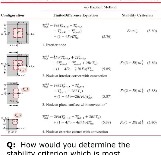
Finite difference equations can be written according to different

geometric boundary conditions. Each boundary condition has a different

stability criterion, so you need to

design ∆t and ∆x based on the most

stringent criterion amongst all of the node geometries you apply.

[

]

[

]

p

n m p

n m p

n m p

n m p

n m p

n

m Fo T T T T Fo T

[image:47.612.50.584.162.676.2]

Table 5.3 in the textbook gives the required finite difference expressions

EXAMPLE: Initially, all nodal points in the diagram below were at 100K. Suddenly, the top side is increased to 500K. Determine the interior nodal temperatures at ∆t, 2∆t, and 3∆t. The

object is 3cm x 3cm and has a

thermal diffusivity of 5x10-6 _m2_/s.

X Y

T = 500 K

T

=

1

0

0

K

T

=

1

0

0

K

T = 100 K

2 3 ₄

5 6 7 8

1

11 12

13

10 9

15 16

14

X Y

T = 500 K

T

=

1

0

0

K

T

=

1

0

0

K

T = 100 K

2 3 ₄

5 6 7 8

1

11 12

13

10 9

15 16

Energy Balance Finite Difference

As with the steady state problems, we can derive the finite difference

equations by writing energy balances around each node assuming all energy transfers into the node of interest

Ein + Egen = Est

   

 

∆ − ⋅

∆ ∆ =

⋅ ∆ ∆ +

+ +

+

+

→

+

→ − →

+

→ −

t T T

y x c

y x q

q q

q q

p n m p

n m p

n m n

m n

m n

m n

m n m n

m n m

, 1

,

, 1 , ,

1 , ,

, 1 ,

, 1

1

1

ρ

&

(m,n+1)

(m,n-1)

(m+1,n) (m-1,n) (m,n)

∆x

∆y

We can also apply numerical methods to solve 1D heat conduction cases for any Fourier number (not only Fo≥0.2)

For example, for a plane:

Solving for Top+1 and substituting

appropriate dimensionless definitions:

(

)

(

)

p

o p

p

o Fo T BiT Fo BiFo T

T +1 = 2 ₁ + _∞ + 1− 2 − 2

∆x

To T1 T2 T3 T4

h, T∞ qconv Est qcond

For node 0 (on the surface):

Q: What is the stability criterion here?

   

 

= ₂

2

dx T d k dt

dT c_p

ρ

st g

conv cond

g

in E q q E E

E& + & = + + & = &

dt dT V c E

q

q_m+→m + _m−→m + 0 = &_st = ρ _p

(

)

t T T

x c

T T

h x

T T

k

p o p

o p

p o p

o p

∆ − ∆

= −

+ ∆

− +

∞

1 1

IMPLICIT METHOD

In an implicit solution, the unknown nodal temperatures at time p+1 are determined relative to other unknown nodal temperatures at time p+1.

! Tm,np appears only in T finite

difference term, not positions

Implicit method is unconditionally stable (i.e. it will always approach a solution) and allows for the selection of any ∆x and ∆t values independently

! preferred if larger time steps are

desired in solution

Q: Compare the interior node

equation for the implicit equations

You can also derive the implicit finite difference equations in the same way as the explicit equations by writing

the positional finite difference terms in terms of Tm,np+1 (backward-difference

approximation) instead of Tm,np

• the energy storage finite difference approximation remains the same

Example: For the 1D surface node Explicit Finite Difference Equation:

Implicit Finite Difference Equation:

The dimensionless number form of the equations may have significantly

different forms since the Top+1 terms

are grouped instead of Top terms

(

)

t T T

x c

T T

h x

T T

k

p o p

o p

p o p

o p

∆ − ∆

= −

+ ∆

− ₊ +

∞

+

+ 1

1 1

1 1

2

ρ

(

)

t T T

x c

T T

h x

T T

k

p o p

o p

p o p

o p

∆ − ∆

= −

+ ∆

− +

∞

1 1

The only known temperature is Top "

all other temperatures are unknown

Since all the nodal T values are

unknown for the present (p+1) time interval, all equations must be solved simultaneously (e.g. Gauss-Seidel or Gaussian elimination methods).

NOTE: You cannot use Excel to solve an implicit problem – Excel calculates based on the explicit method.

Thus, while the explicit method is

much easier to calculate, the implicit calculation is inherently stable (i.e. no stability criterion need be assessed)

NOTE: There is actually a 3rd _method

which is typically favoured (the

EXAMPLE: An AISI 302 stainless steel plate is surrounded by an insulating block as shown and is initially at a uniform temperature of

50°C. The surface is exposed to a convective fluid with T∞ = 50°C and h = 30W/m2K. The

surface plate is suddenly exposed to a radiant heat flux of 20 kW/m2_{. (Final Exam Question, 2011)}

(a) Write the explicit finite difference

equations for nodes 1, 2, 3, and 4.

(b) Write the implicit finite difference equation

for node 1 only.

(c) Calculate the temperature at node 1 at

the maximum possible time increment for which a stable solution can be achieved.

2 cm

4 cm a

b c

d

y

x

PROBLEM SOLVING HEURISTIC FOR HEAT CONDUCTION:

1. Start from the general equation,

(

k T

)

q

dt dT

C_P = ∇⋅ ∇ + &

ρ

(rect., cylind., spherical co-ords) 2. Simplify

# Steady-state? # 1-D, 2-D?

# Constant properties? # Heat generation/loss?

3. Identify the appropriate B.C (and I.C. if required)

# Given temperature # Symmetry / perfect

insulation

# Given heat flux # Convection

4. Solve by: