FORWARD RATE VOLATILITIES, SWAP RATE VOLATILITIES, AND THE IMPLEMENTATION OF THE LIBOR MARKET MODEL
John Hull and Alan White
Joseph L. Rotman School of Management University of Toronto
August, 1999
Abstract
FORWARD RATE VOLATILITIES, SWAP RATE VOLATILITIES, AND THE IMPLEMENTATION OF THE LIBOR MARKET MODEL
The most popular over-the-counter interest rate options are interest rate caps/floors and European swap options. The standard market models for valuing these instruments are versions of Black’s (1976) model. This model was originally developed for valuing options on commodity futures, but has found many other applications in financial engineering. When Black’s model is used to value a caplet (one element of an interest rate cap), the underlying interest rate is assumed to be lognormal. When it is used to value European swap options, the underlying swap rate is assumed to be lognormal. Researchers such as Jamshidian (1997) have shown that the cap/floor market model and the European swap option market model are each internally consistent in the sense that they do not permit arbitrage opportunities. However, they are not exactly consistent with each other.
In recent years Brace, Gatarek, and Musiela (1997), Jamshidian (1997), and Miltersen, Sandmann, and Sondermann (1997) have developed what has become known as the LIBOR market model. This is an extension of the Heath, Jarrow, and Morton (HJM) (1992) model. Whereas the HJM model describes the behavior of instantaneous forward rates expressed with continuous compounding, the LIBOR market model describes the behavior of the forward LIBOR rates underlying caps and floors, with the usual market conventions being used for compounding (that is, the compounding period equals the tenor of the rate). Brace, Gatarek, and Musiela (1997) show that the LIBOR market model overcomes some technical existence problems associated with the lognormal version of the HJM model.
Glasserman (1997) propose an approach involving a stochastic recombining tree. Longstaff and Schwartz (1998) assume that the value of an option, if not exercised, is a simple function of variables observed at the exercise date in question. These approaches make it feasible to use the LIBOR market model to value instruments such as Bermudan swap options, which are becoming increasingly popular.
This paper develops and tests an analytic approximation for pricing European swap options under the LIBOR market model and its extensions. This approximation makes it possible to translate the volatility skews observed for caps into volatility skews for European swap options. It also simplifies the process of calibrating the LIBOR market model to the market prices of caps and swap options.
1. THE STANDARD MARKET MODELS FOR CAPS AND SWAPTIONS In this section we explain the standard market models for pricing caps and European swap options. We will use the result of Harrison and Kreps (1979) that, in any market where there is no arbitrage, for any given numeraire security whose price is g(t), there exists a measure for which f(t)/g(t) is a martingale for all security prices f(t). We will denote this measure by M{g(t)}.
1.1 Interest Rate Caps
Consider a cap with strike rate Rc and reset dates at timest1, t2, . . ., tN with a final
payment date tN+1. Define δi =ti+1−ti and Ri as theδi-maturity rate observed at time ti and expressed with a compounding period of δi (1 ≤i ≤ N). The cap is a portfolio of N caplets. The ith caplet provides a payoff at time ti+1 equal to
Lcδimax[Ri−Rc, 0] (1)
where Lc is the principal.
Define P(t, T) as the price of a discount bond paying off $1 at time T. To value the
ith caplet we use P(t, ti+1) as the numeraire. Under the measure, M{P(t, ti+1)}
f(t)
P(t, ti+1)
is a martingale for all security prices f(t). Hence
f(0)
P(0, ti+1)
=Ei+1
f(t)
P(t, ti+1)
(2)
where Ei+1 denotes expectations under M{P(t, ti+1)}.
By setting f(t) =P(t, ti)−P(t, ti+1) in equation (2), we see that
Fi(0) =Ei+1(Ri) (3)
whereFi(t) is the forward interest rate for the period (ti, ti+1) observed at timet. Equation
By setting f(t) equal to the price of the ith caplet and noting that P(ti+1, ti+1) = 1,
we see from equation (2) that
f(0) =P(0, ti+1)Ei+1[f(ti+1)]
or
f(0) =P(0, ti+1)LcδiEi+1[max(Ri−Rc, 0]
Assuming Ri is lognormal, with the standard deviation of ln(Ri) equal to σi
√
ti, this
becomes
f(0) =P(0, ti+1)Lcδi[Ei+1(Ri)N(d1)−RcN(d2)]
where
d1 =
ln[Ei+1(Ri)/Rc] +σi2ti/2 σi
√
ti
d2 =d1−σi
√
ti
and N(x) is the cumulative normal distribution function. Substituting from equation (3) gives the standard market model for valuing the caplet:
f(0) =P(0, ti+1)Lcδi[Fi(0)N(d1)−RcN(d2)] (4)
where
d1 =
ln[Fi(0)/Rc] +σ2iti/2
σi√ti d2 =d1−σi
√
ti
Similarly the standard market model for valuing the ith element of a floor is
f(0) =P(0, ti+1)Lcδi[RcN(−d2)−Fi(0)N(−d1)] (5)
The variableσi is often referred to the volatility of the (ti, ti+1) forward rate. In fact,
the forward rate during the life of the caplet. This point is important for understanding of the model in the next section. To avoid confusion with variables introduced in the next section, we will refer to σi as the spot volatility of the (ti, ti+1) rate, or the spot volatility
of the ith caplet.
In practice brokers usually quote what is known as a flat volatility for a cap. This is a volatility which, if used as the spot volatility for all the underlying caplets, reproduces the cap’s market price. When flat volatilities for all cap maturities are available or can be estimated, spot volatilities can be calculated. The procedure is to use the flat volatilities and equation (4) to calculate cap prices, deduce caplet prices by subtracting one cap price from the next, and then imply the spot volatilities from these caplet prices using equation (4).
1.2 European Swap Options
We now move on to consider a European swap option. Suppose that the underlying swap lasts from timetn to timetN+1 and the strike rate isRs. The swap reset dates aretn, tn+1, . . ., tN and the corresponding payment dates are tn+1, tn+2, . . ., tN+1, respectively.
We define
An,N(t) =
N
X
i=n
δiP(t, ti+1)
where as before P(t, T) is the price of a discount bond paying off $1 at time T and
δi = ti+1 −ti. We will denote by Sn,N(t) (0 ≤ t ≤ tn) the forward swap rate. This is
the fixed rate which, when it is exchanged for floating in a forward start swap, causes the value of the swap to be zero. An expression for Sn,N(t) is
Sn,N(t) =
P(t, tn)−P(t, tN+1)
An,N(t)
(6)
can be viewed as providing payments of
Lsδimax(Rn,N −Rs, 0)
at times ti+1 for n≤i ≤N where Ls is the swap principal. The value of the swap option
at time tn is
LsAn,N(tn) max(Rn,N −Rs, 0) (7)
We will value the European swap option at time zero usingAn,N(t) as the numeraire.
Under the measure M{An,N(t)}
f(t)
An,N(t)
is a martingale for all security prices f(t). Hence
f(0)
An,N(0)
=EA
f(tn)
An,N(tn)
(8)
whereEA denotes expectations under the measure. By settingf(t) =P(t, tn)−P(t, tN+1)
in equation (8) we see that
Sn,N(0) =EA[Sn,N(tn)] =EA(Rn,N) (9)
The forward swap rate, therefore, equals the expected future swap rate under the measure. We now set f(t) equal to the value of the swap option. Equation (8) gives
f(0) =An,N(0)EA
f(tn)
An,N(tn)
Substituting for f(tn) from equation (7) we obtain
f(0) =LsAn,N(0)EA[max(Rn,N −Rs, 0)]
Assuming Rn,N is lognormal with the standard deviation of ln(Rn,N) equal to σn,N√tn
this becomes
where
d1 =
ln[EA(Rn,N)/Rs] +σn,N2 tn/2
σn,N√tn d2 =d1−σn,N
√
tn
Substituting from equation (9) gives the standard market model for valuing the swap option
f(0) =LsAn,N(0)[Sn,N(0)N(d1)−RsN(d2)] (10)
where
d1 =
ln[Sn,N(0)/Rs] +σn,N2 tn/2
σn,N√tn d2 =d1−σn,N
√
tn
Similarly the standard market model for valuing a swap option that gives the holder the right to receive fixed and pay floating is
f(0) =LsAn,N(0)[RsN(−d2)−Sn,N(0)N(−d1)] (11)
The variable σn,N is usually referred to as the forward swap rate volatility. As in the case of interest rate caps, we emphasize that the model does not require the forward swap rate’s volatility to be constant between times 0 and tn. It is sufficient for its average
variance rate to be σ2
n,N during this period. We will refer toσn,N as the spot volatility of
2. THE LIBOR MARKET MODEL
In this section we discuss the development and implementation of the LIBOR market model. Our notation is consistent with Section 1.1. We consider a cap with reset dates at times t1, t2, . . . , tn and a final payment date tn+1. We define t0 = 0, δi = ti+1 − ti
(0≤i≤n), and
Fi(t): Forward rate observed at time t for the period (ti, ti+1), expressed with a
com-pounding period ofδi
P(t, T): Price at time t of a zero-coupon bond that provides a payoff of $1 at time T m(t): Index for the next reset date at time t. This means that m(t) is the smallest
integer such thatt ≤tm(t).
p: Number of factors
ζi,q: qth component of the volatility of Fi(t) (1≤q ≤p)
vi,q: qth component of the volatility of P(t, ti) (1≤q ≤p)
We assume that the components to the volatility are independent. (This is not re-strictive since they can be orthogonalized.) The processes followed by Fi(t) and P(t, ti) are:
dFi(t) =. . . dt+
p
X
q=1
ζi,q(t)Fi(t)dzq (12)
dP(t, ti) =. . . dt+
p
X
q=1
vi,q(t)P(t, ti)dzq
where the dzq are independent Wiener processes and the drifts depend on the measure. In
this section and the next, we will assume a model where ζi,q(t) is a function only of time.
The bond price volatility, vi,q(t), is in general stochastic in this model.
We will use as numeraire a money market account that is invested at time t0 for a
period δ0, reinvested at time t1 for a period δ1, reinvested at time t2 for a period δ2, and
chosen measure
f(t)
P(t, tm(t))
is a martingale for all security prices f(t) when tm(t)−1 ≤t≤tm(t) so that
f(tm(t)−1)
P(tm(t)−1, tm(t))
=Em(t)
f(t
m(t))
P(tm(t), tm(t))
or
f(tm(t)−1) =P(tm(t)−1, tm(t))Em(t){f(tm(t))}
where Em(t) denotes expectations under M{P(t, tm(t))} This equation shows that the
chosen measure allows us to discount expected values one accrual period at a time when security prices are valued. Since cash flows and early exercise opportunities usually occur only on reset dates, this is an attractive feature of the measure.
It can be shown that theqth component of the market price of risk under the measure M{P(t, tj)} is vj,q for all j. [See for example, Jamshidian (1997).] As shown in Section 1.1, under the measure M{P(t, ti+1)} Fi(t) is a martingale so that its drift is zero. It
follows that the expected growth rate of Fi(t) under the M{P[t, tm(t)]} measure is
p
X
q=1
ζi,q(t)[vm(t),q(t)−vi+1,q(t)]
so that
dFi(t)
Fi(t)
=
p
X
q=1
ζi,q(t)[vm(t),q(t)−vi+1,q(t)]dt+ p
X
q=1
ζi,q(t)dzq (13)
The relationship between forward rates and bond prices is
P(t, tj)
P(t, tj+1)
= 1 +δjFj(t)
Using this in conjunction with Ito’s lemma leads to
vj,q(t)−vj+1,q(t) =
δjFj(t)ζj,q(t)
Repeated application of this result gives
vm(t),q(t)−vi+1,q(t) = i
X
j=m(t)
δjFj(t)ζj,q(t) 1 +δjFj(t)
and substituting into equation (13) we see that the process followed by Fi(t) under the
measure M{P(t, tm(t))}is
dFi(t) Fi(t) =
i
X
j=m(t)
δjFj(t)Pp
q=1ζj,q(t)ζi,q(t)
1 +δjFj(t) dt+
p
X
q=1
ζi,q(t)dzq (15)
When we take limits allowing theδi’s to approach zero, this becomes
dF(t, T) =
p
X
q=1
ζq(t, T)F(t, T)
Z T
τ=t
ζq(t, τ)F(t, τ)dτ + p
X
q=1
ζq(t, T)F(t, T)dzq
where the notation is temporarily changed so that F(t, T) is the instantaneous forward rate at timet for maturityT and ζq(t, T) is theqth component of the volatility of F(t, T).
This is the HJM result. The HJM model is, therefore, a limiting case of the LIBOR market model.
2.1. Determining Forward Rate Volatilities
We now simplify the model by assuming thatζi,q(t) is a function only of the number of whole accrual periods between the next reset date and time ti. Define λj,q as the value of ζi,q(t) when there arej such accrual periods. This means that
ζi,q(t) =λi−m(t),q (16)
Define Λj as total volatility of a forward rate when there are j whole accrual periods
until maturity so that
Λj =
v u u t p X q=1 λ2 j,q (17)
The Λ’s can be calculated from the spot volatilities, σi, used to value caplets in equation
(4). Equating variances we must have:
σi2ti =
i
X
j=1
This allows the Λ’s to be obtained inductively. For example, ifσ1,σ2, andσ3 are 20%, 22%
and 21%, respectively and the δi are all equal, Λ0 = 20%, Λ1=23.83% and Λ2 = 18.84%
Similarly to Rebonato (1999), we favor a two step approach to obtaining theλj,q. The first stage is to determine the Λj from market data; the second stage is to use historical
data to determine the λj,q from the Λj. Rebonato (1999) proposes a way of determining
the λj,q from the Λj to provide as close a fit as possible to the correlation matrix for
the Fj(t) (1 ≤ j ≤ N). As Rebonato points out, the approach gives similar results to
a principal components analysis. If output from a principal components analysis on the
Fj(t) (1 ≤ j ≤ N) is available, we can use it in a direct way to determine values of λj,q. Suppose that αi,q is the factor loading for the ith forward rate and the qth factor, and sq
is the standard deviation of the qth factor score.1 If the number of factors being used, p, were equal to N, the number of forward rates, it would be correct to set
λj,q =αj,qsq
for 1≤j, q ≤N. When p < N, the λj,q can be scaled so that the relationship in equation (17) holds. This involves setting
λj,q = qΛjsqαj,q Pp
q=1s2qα2j,q
(19)
1 The principal components analysis model is
∆Fj =
N
X
q=1
αj,qxq
where
N
X
j=1
αj,q1αj,q2
equals 1 when q1 = q2 and zero when q1 6=q2. The variable sq is the standard deviation
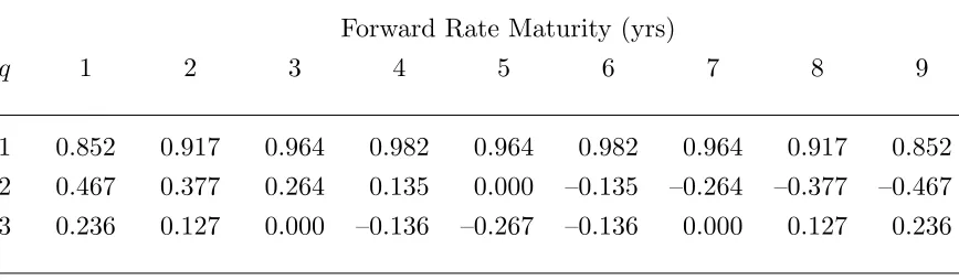
Table 1 shows the λj,q/Λj values used for the analyses reported in this paper. These
are based on equation (19) and data that is typical of the results obtained from a principal components analysis. The first factor corresponds to a roughly parallel shift in the yield curve; the second factor corresponds to a twist in the zero curve where short maturity rates move in one direction and long maturity rates move in the opposite direction; the third factor corresponds to a bowing of the zero curve where short and long maturity rates move in one direction and intermediate maturity rates move in the opposite direction. 2.2. Implementation of the Model
From equation (15), the process for Fi(t) under the measureM{P(t, tm(t))} is
dFi(t) Fi(t) =
i
X
j=m(t)
δjFj(t)P p
q=1λj−m(t),qλi−m(t),q
1 +δjFj(t) dt+
p
X
q=1
λi−m(t),qdzq (20)
or
dlnFi(t) = i
X
j=m(t)
"
δjFj(t)Pp
q=1λj−m(t),qλi−m(t),q
1 +δiFi(t) −
p
X
q=1
λ2
i−m(t),q
2 # dt+ p X q=1
λi−m(t),qdzq
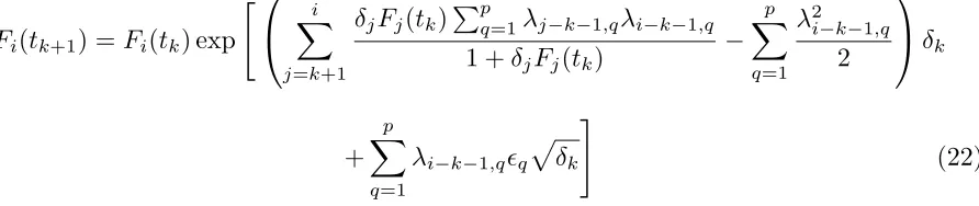
(21) An approximation that simplifies the Monte Carlo implementation of the model is that the drift of lnFi is constant between times tk and tk+1 so that
Fi(tk+1) =Fi(tk) exp
"
i
X
j=k+1
δjFj(tk)Pp
q=1λj−k−1,qλi−k−1,q
1 +δjFj(tk) −
p
X
q=1
λ2i−k−1,q
2
δk
+
p
X
q=1
λi−k−1,qq
p
δk
#
(22)
where q are independent random samples from standard normal distributions.
M{P(t, tm(t))}measure. The value ofFi(ti) is the realized rate for the time period between ti and ti+1 and enables the caplet payoff at time ti+1 to be calculated. This payoff is
discounted to time zero using Fj(tj) as the discount rate for the interval (tj, tj+1). The
estimated caplet value is the mean of the discounted payoffs.
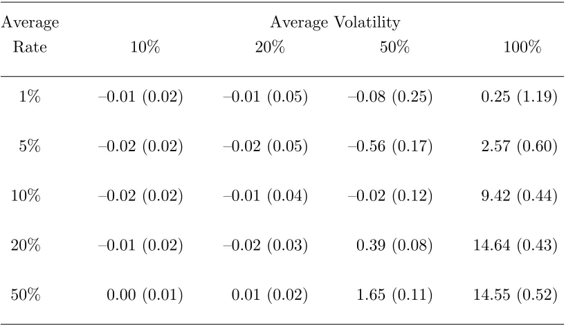
We have carried out the test just described for a variety of term structures, volatility structures, strike rates, and number of factors. Typical results are shown in Table 2. This table is based on an upward sloping term structure, a humped volatility structure similar to that observed in the market, and at-the-money caplets (that is, caplets where the strike rate equals the forward rate). Three factors and 200,000 Monte Carlo trial were used. The δi were set equal to one year.2 This table shows the mean and standard error
of the difference between the true spot volatility of a caplet and the volatility implied from the caplet price calculated using the LIBOR market model, with both volatilities being measured in percent. The results shown are for the fifth caplet. Similar results are obtained for other caplets, other term structures, other volatility structures, and other choices for the strike rate and the number of factors. The average interest rates reported in Table 2 are the arithmetic average the zero rates for maturities of 1, 2, 3,. . ., 10 years. The average volatilities are similarly the arithmetic average of the spot volatilities between one and ten years.
Table 2 shows that, for the volatility and interest rate environments that are typically encountered in North America and Europe, the implementation of the model in equation (22) gives very accurate results. Consider, for example, the case where the average interest rate is 5% and the average volatility is 20%. If the true spot volatility for a particular caplet isV%, Table 2 shows that we can be 95% certain that the equation (22) implementation of the LIBOR market model is implicitly assuming a spot volatility between V −0.12% and
2 The error in equation (22) is likely to increase with the length of the accrual period.
V + 0.08%.3 As the volatility increases the approximation in equation (22) works less well. In some countries (for example, Japan), very low short-term interest rates are sometimes coupled with spot volatilities as high as 100% for short-maturity caplets. Table 2 shows that the approximation in equation (22) may not be appropriate in these cases.4
3 To put this result in perspective, the bidoffer spread for the flat volatilities quoted
by brokers in the U.S. is typically 0.5%.
4 The lognormal LIBOR market model described here may itself be inappropriate in
3. APPROXIMATE PRICING OF EUROPEAN SWAP OPTIONS
In this section we present an approximate, but very accurate, procedure for pricing European swap options in the LIBOR market model. Other approximations have been suggested by Brace, Gatarek, and Musiela (1997) and Andersen and Andreasen (1997). Our approach is similar in spirit to that of Andersen and Andreasen, but is much easier to implement than either of the other two approaches. It is motivated by the observation that when forward LIBOR rates are lognormal, swap rates are approximately lognormal and approximately linearly dependent on forward LIBOR rates.
As in Section 1.2 we consider an option on a swap lasting from tn to tN+1 with reset
dates at times tn, tn+1, . . ., tN. Initially we assume that the reset dates for the swap
coincide with the reset dates for caplets underlying the LIBOR market model. Later we relax this assumption.
The relationship between bond prices and forward rates is
P(t, tk)
P(t, tn) =
k−1
Y
j=n
1 1 +δjFj(t)
for k ≥n+ 1. It follows that the formula for the forward swap rate in equation (6) can be written
Sn,N(t) =
1−QN
j=n
1 1+δjFj(t) PN
i=nδi
Qi
j=n
1 1+δjFj(t)
(We employ the convention that empty sums equal zero and empty products equal one.) Equivalently
Sn,N(t) =
QN
j=n[1 +δjFj(t)]−1
PN
i=nδi
QN
j=i+1[1 +δjFj(t)]
(23)
or
lnSn,N(t) = ln
N
Y
j=n
[1 +δjFj(t)]−1
−ln N X
i=n δi
N
Y
j=i+1
[1 +δjFj(t)]
so that
1
Sn,N(t)
∂Sn,N(t) ∂Fk(t) =
δkγk(t)
where
γk(t) =
QN
j=n[1 +δjFj(t)]
QN
j=n[1 +δjFj(t)]−1
−
Pk−1
i=nδi
QN
j=i+1[1 +δjFj(t)]
PN
i=nδi
QN
j=i+1[1 +δjFj(t)]
From Ito’s lemma the qth component of the volatility of Sn,N(t) is N
X
k=n
1
Sn,N(t)
∂Sn,N(t)
∂Fk(t)
ζk,q(t)Fk(t)
or
N
X
k=n
δkζk,q(t)Fk(t)γk(t) 1 +δkFk(t) The variance rate of Sn,N(t) is therefore
p
X
q=1
" N X
k=n
δkζk,q(t)Fk(t)γk(t) 1 +δkFk(t)
#2
Assuming, as in Section 2.1 that ζk,q(t) =λk−m(t),q, the variance rate of Sn,N(t) is
p
X
q=1
" N X
k=n
δkλk−m(t),qFk(t)γk(t)
1 +δkFk(t)
#2
This expression is in general stochastic showing that when the forward rates underlying caplets are lognormal, swap rates are not lognormal. For the purposes of evaluating the expression we assume that Fk(t) = Fk(0). This means that the volatility of Sn,N(t) is constant within each accrual period and the swap rate is lognormal. The average variance rate of Sn,N(t) between time zero and time tn is
1
tn n−1
X j=0 δj p X q=1 " N X
k=n
δkλk−j−1,qFk(0)γk(0)
1 +δkFk(0)
#2
The spot swap option volatility is therefore v u u u t 1 tn n−1
X j=0 δj p X q=1 " N X
k=n
δkλk−j−1,qFk(0)γk(0)
1 +δkFk(0)
#2
(24)
3.1 Non-Matching Accrual Periods
The accrual periods for the swaps underlying broker quotes for European swap options do not always match the accrual periods for the caps and floors underlying broker quotes. For example, in the United States the benchmark caps and floors have quarterly resets while the swaps underlying the benchmark European swap options have semiannual resets. To accommodate this, we now extend the analysis to the situation where each swap accrual period includes M cap accrual periods where M ≥1 is an integer.
Assume that δn, δn+1, . . ., δN are the swap accrual periods and that within the ith
swap accrual period the cap accrual periods are i,1, i,2, . . ., i,M with
δi = M
X
m=1
i,m
Assume that Gi,m(t) is the forward rate observed at time t for the i,m accrual period. Since
1 +δiFi(t) =
M
Y
m=1
[1 +i,mGi,m(t)]
∂Fi(t)
∂Gi,m(t)
= i,m[1 +δiFi(t)]
δi[1 +i,mGi,m(t)]
The qth component of the volatility of Sn,N(t) is
N
X
k=n M
X
m=1
1
Sn,N(t)
∂Sn,N(t)
∂Gk,m(t)ζk,m,q(t)Gk,m(t)
where ζk,m,q is the qth component of the volatility of Gk,m(t). Using
∂Sn,N(t) ∂Gi,m(t) =
∂Sn,N(t) ∂Fi(t)
∂Fi(t) ∂Gi,m(t)
we find that the estimate in equation (24) of the spot swap option volatility is
v u u u t 1 tn n−1
X j=0 δp p X q=1 " N X
k=n M
X
m=1
δkλk−j−1,m,qGk,m(0)γk,m(0)
1 +δkFk(0)
#2
where
γk,m(t) =γk(t)
k,m[1 +δkFk(t)] δk[1 +k,mGk,m(t)]
and λj,m,q is the qth component of the volatility of Gi,m(t) when i−m(t) =j. 3.2. Accuracy of Approximation
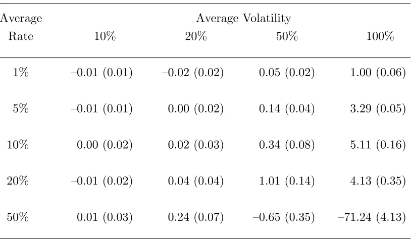
To assess the accuracy of the assumption that forward rates are constant in equations (24) and (25) we performed tests analogous to those described in section 2.2 for testing the accuracy of caplet pricing. Typical results are shown in Table 3. These are based on 200,000 Monte Carlo trials of equation (22) usingδi= 1, an upward sloping term structure,
a humped volatility structure similar to that observed in the market, and three factors. The table shows the mean and standard error of the difference between the estimates of the spot volatility of swap options calculated from the LIBOR market model and estimates of the spot volatilities of swap options calculated from the approximation in Section 3.1. The results shown are for a 5×5 swap option (that is, a five year option to enter into a five year swap) with the underlying swap being reset annually. The strike rates are at-the money (that is, the strike rate equals the forward swap rate). Similar results are obtained for other swap options, other strike rates, other interest rate term structures, other volatility structures, and other choices for the number of factors. Average interest rates and average volatilities are defined as in Table 2.
reported for caps in Table 2. For situations where the errors in both Tables 2 and 3 are low, we can therefore assume that the approximation in Section 3.1 works well.
The results show that the approximation in Section 3.1 works well for the interest rates and volatilities normally encountered in North America and Europe. Consider, for example, the situation where interest rates average 5% and volatilities average 20%. Even after the equation (22) error is taken into account, the error in the approximation of the 5×5 swap option volatility is likely to be less than 0.1%. This translates into a pricing error of less than $2 per $1 million of principal.5
5 Brace, Gatarek, and Musiela (1997) report errors for a 5 × 5 swap option of about
4. MODELING VOLATILITY SKEWS
The volatility skew for equities has been well documented by authors such as Jackwerth and Rubinstein (1996). As pointed out by Andersen and Andreasen (1997), caps and floors exhibit a similar volatility skew to equities. The lower the strike price, the higher the volatility implied from the standard market model in equations (4) and (5). Some brokers do provide quotes for caps that are not at the money, but there is very little data on the pricing of non-at-the-money European swap options. It is, therefore, of interest to investigate how cap volatility skews can be converted to swap option volatility skews.
As shown by Andersen and Andreasen (1997), the LIBOR market model can be ex-tended to incorporate volatility skews. We consider the version of their model where the process for forward rates in equation (12) is replaced by a CEV model
dFi(t) =. . .+
p
X
q=1
ζi,q(t)Fi(t)αdzq (26)
where α is a positive constant. We generalize the notation in Section 2.1 to define λj,q as the value of ζi,q(t) in this model when there are j whole accrual periods between time t
and time ti. This means that
ζi,q(t) =λi−m(t),q
The process for forward rates in equation (20) becomes
dFi(t)
Fi(t)α = i
X
j=m(t)
δjFj(t)αPp
q=1λj−m(t),qλi−m(t),q
1 +δjFj(t) dt+
p
X
q=1
λi−m(t),qdzq
or
dQi(t) =
i
X
j=m(t)
"
δjFj(t)αPp
q=1λj−m(t),qλi−m(t),q
1 +δjFj(t)
−
p
X
q=1
αFi(t)α−1λ2i−m(t),q
2 # dt + p X q=1
λi−m(t),qdzq
where
Qi(t) =
1
1−αFi(t)
Analogously to the approach taken in section 2.2 in arriving at equation (22), we assume that the drift of Qi(t) is constant between times tj and tj+1 to get
Qi(tk+1) =Qi(tk)+δk
i
X
j=k+1
"
δjFj(tk)αPp
q=1λj−k−1,qλi−k−1,q
1 +δjFj(tk)
−
p
X
q=1
αFi(tk)α−1λ2i−k−1,q
2 # + p X q=1
λi−k−1,qq
p
δk (27)
We define Λj by
Λj =
v u u t p X q=1
λ2j,q (28)
and σi by:
σi2 = 1
ti i
X
j=1
Λ2i−jδj−1 (29)
These definitions are consistent with equations (17) and (18) in Section 2. However, our notation is now more general than in Section 2. In equations (17) and (18) the Λ’s and
σ’s were volatilities whereas here they are volatilities only when α = 1.
Andersen and Andreasen (1997) show that the process in equation (26) implies that the price of the ith caplet is
P(0, ti+1)Lcδi[Fi(0)−Fi(0)χ2(a, b+ 2, c)−Rcχ2(c, b, a)] (30)
when 0< α <1 and
P(0, ti+1)Lcδi[Fi(0)−Fi(0)χ2(c,−b, a)−Rcχ2(a,2−b, c)] (31)
when α >1 where
a = R
2(1−α)
c
(1−α)2σ2
iti
; b= 1
1−α; c=
Fi(0)2(1−α)
(1−α)2σ2
iti
and χ2(z, v, k) is the cumulative probability that a non-central chi-squared distribution with non-centrality parameter v and k degrees of freedom is less than z. The price of the
ith floorlet is
when 0< α <1 and
P(0, ti+1)Lcδi[Rc−Fi(0)χ2(c,−b, a)−Rcχ2(a,2−b, c)]
when α > 1. When α = 1, equations (4) and (5) give the caplet and floorlet prices, respectively.
Andersen and Andreasen (1997) also show that skews for swap rates can be analyzed in an analogous way to skews for forward rates. Suppose that the swap rate considered in Section 1.2 follows a process of the form
dSn,N(t) =. . .+
p
X
q=1
ηq,n,N(t)Sn,N(t)βdzq (32)
where β is a positive constant. We define σn,N by
σn,N2 = 1
tn
Z tn
τ=0
p
X
q=0
ηq,n,N(τ)2dτ
In the special case where β = 1 this is the same as the σn,N in Section 1.2. The value of the European swap option that gives the holder the right to pay fixed is
LsAn,N(0)[Sn,N(0)−Sn,N(0)χ2(e, f + 2, g)−Rsχ2(g, f, e)] (33)
when 0< α <1 and
LsAn,N(0)[Sn,N(0)−Sn,N(0)χ2(g,−f, e)−Rsχ2(e,2−f, g)] (34)
when α >1 where
e = R
2(1−β)
s
(1−β)2σ2
n,Ntn
; f = 1
1−β; g=
Sn,N(0)2(1−β)
(1−β)2σ2
n,Ntn
The value of the European swap option that gives the holder the right to pay floating is
when 0< α <1 and
LsAn,N(0)[Rs−Sn,N(0)χ2(g,−f, e)−Rsχ2(e,2−f, g)] (36)
when α >1. When β = 1, equations (10) and (11) give the swap option price.
In Section 3 we showed that, for the volatility and interest rate environments normally encountered, whenα = 1 in equation (26) it is reasonable to assume that swap rates follow the process in equation (32) with β = 1. We now hypothesize that a more general version of this result holds. We suppose that, when rates follow the process in equation (26), to a reasonable approximation swap rates follow the process in equation (32) with β =α. This is an attractive hypothesis. A similar analysis to that in Section 3.1 shows that it leads to
σn,N being approximately equal to6
Sn,N(0)1−β v u u u t
1
tn n−1
X
j=0
δp p
X
q=1
" N X
k=n M
X
m=1
δkλk−j−1,m,qGk,m(0)αγk,m(0)
1 +δkFk(0)
#2
(37)
where Sn,N(0) is given by equation (23).
To test the hypothesis we compared European swap option prices calculated from: 1. A Monte Carlo simulation of the extended LIBOR market model using the
approxi-mation in equation (27); and
2. Equation (35) or (36) combined with the estimate ofσn,N in equation (37) andβ =α. Typical results, based on 100,000 antithetic simulation trials, are shown in Table 4. These are for a 3×3 European swap option in which the holder has the right to pay floating. The average ten year interest rate is 5% and the average ten year volatility is
6 A more general version of the hypothesis is that swap rates follow the process in
20%. The term structure is upward sloping and the volatility structure is humped. The tenor of the caplets underlying the model is three months and the swap underlying the European swap option is reset semiannually.
The results for α6= 1 are not quite as good as those for α = 1, but they are still quite acceptable. The largest errors (about 0.4%) are for deep-in-the-money swap options. The prices of these options are relatively insensitive to volatilities and so these errors are not a cause for serious concern.
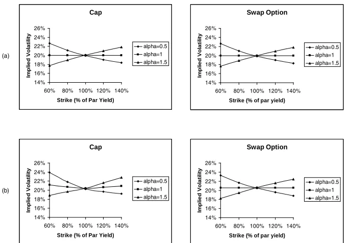
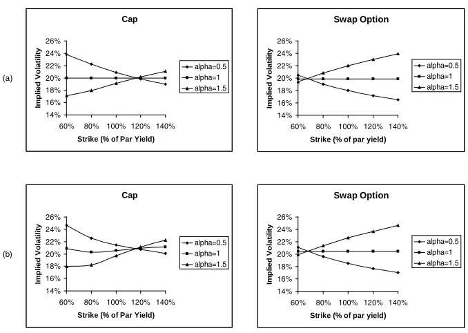
Figures 1 and 2 use the results in this section to compare cap volatility skews with swap option volatility skews in a variety of situations. The figures show flat volatilities for a five year cap and spot volatilities for 3×3 European swap option. In Figure 1 the term structure is flat at 5%; in Figure 2 it is upward sloping. Three different values of α
are considered. The cap is reset quarterly; the swap underlying the swap option is reset semiannually. In Figures 1(a) and 2(a) the volatility structure is flat at 20%. In Figures 1(b) and 2(b) it has a hump similar to that observed in the market.
The figures show that care must be exercised in interpreting cap volatility skews. The latter are affected by the way in which the flat volatilities quoted by brokers are calculated. A flat volatility is the volatility that, when applied to all caplets, produces the market price. It is, therefore, a complex non-linear function of true caplet spot volatilities. As shown by the cap volatilities for the α = 1 case in Figure 1(b), the function depends on the strike price. (If the function did not depend on the strike price, these cap volatilities would be the same for all strike prices.)
When the term structure is upward sloping (Figure 2), the cap results are affected by the fact that the moneyness of the early caplets is less than that of the later caplets. Consider, for example, the case where the volatility structure is flat and the cap is at the money (Figure 2a). The short maturity caplets are out of the money and the long maturity caplets are in the money. When α = 1 they are all priced with the same volatility. When
maturity caplets are priced with relatively high volatilities. This increases the value of the cap. When α = 1.5 the short maturity caplets are priced with relatively high volatilities and long maturity caplets are priced with relatively low volatilities. This decreases the value of the cap.
5. APPLICATIONS OF THE MODEL
There are two main applications of the model in Section 4. The first is to valuation and marking to market of non-standard interest rate derivatives. The second is to the valuation and marking to market of non-at-the-money European swap options. We will discuss both of these applications in this section. We will use for illustration U.S. data on caps and European swap options for August 12, 1999, kindly supplied to us by a major investment bank. The data was compiled by averaging mid-market quotes from a number of different brokers.7 It was used by the bank to mark to market its portfolio of interest rate derivatives on August 12, 1999. The cap data consists of 133 flat volatility quotes where the strike prices range from 3% to 10% and the cap lives range from one to ten years. The swap data consists of at-the-money volatility quotes for a range of different option maturities and swap lives. The caps were reset quarterly and the swaps were reset semiannually. The zero curve on August 12, 1999 was upward sloping with short rates approximately 5.3% and long rates approximately 7.2%.
The first step in implementing the model in Section 4 is to estimate α. This can be done by simultaneously estimatingαand the Λj from cap prices.8 We search for the values
of α and the Λj that minimize the root mean square cap pricing error
v u u t
1
K K
X
i=1
(ui−vi)2 (38)
where K is the number of caps for which market data is available, ui is the market price of theith cap calculated from the broker (flat) volatility quotes using equation (4), andvi
is the model price of the ith cap calculated using equations (30) and (31).
7 Because different brokers quote data in different ways, some judgment must be used
in averaging quotes.
8 Note that cap prices depend only on the Λ
j in equation (28) not on the way in
The best fit value of α on August 12, 1999 was found to be 0.716. This value of
α reflects a situation where quoted cap volatilities declined, in absolute terms, by 3% to 4% as the strike price increased from 3% to 10%. The best fit values of the Λj obtained
from this analysis of cap prices are shown in the Caps column of Table 5. As indicated by the table, we assumed a step function for Λj.9 The reflects the fact that the only cap
maturities for which we had data were 1, 2, 3, 4, 5, 7, and 10 years.
A natural application of the LIBOR market model, once it has been calibrated to plain vanilla caps in the way just described, is to the valuation of non-standard cap products. Hull (2000) examines three such products: ratchet caps, sticky caps, and flexi caps. In a ratchet cap the strike rate for a caplet equals the LIBOR rate at the previous reset date plus a spread. In a sticky cap it equals the previous capped LIBOR rate plus a spread. In a flexi cap there is an upper bound to the total number of caplets that can be exercised. Hull finds that the prices of all three types of nonstandard caps are dependent on the number of factors. This is because their payoffs, unlike those of a plain vanilla cap, depend on the joint behavior of two or more forward rates. Hull’s analysis used Monte Carlo simulation in conjunction with equation (22) to price the instruments. To investigate the impact of volatility skews we could carry out a similar analysis using Monte Carlo simulation in conjunction with equation (27).
To value non-standard swap option products, such as Bermudan swap options, the most appropriate procedure would seem to be to setα equal to its best fit value calculated from caps and choose the Λj so that they fit broker quotes on at-the-money European
swap options. We did this using 30 swap option quotes where the option maturity ranged from 0.5 years to 5 years and the swap life ranged from 1 to 5 years. We used a three factor model, determining the λj,q from the Λj as indicated in Table 1. The results are
9 When finding best fit Λ
j values we imposed some smoothness constraints to avoid
shown in the Swap Option column of Table 5.
If the three-factor extended LIBOR market model were perfect, we would of course obtain the same parameter values regardless of the calibrating instruments being used. The reality is that all derivative models even those involving several factors have to be fine tuned to reflect the use to which they are being put. Table 5 shows that the Λj
values obtained by fitting the model to swap options are different from those obtained by fitting it to caps. Specifically, the Λ’s implied from swap options are less humped than those implied from caps. This appears to be because the pricing of options on one and two year swaps does not fully reflect the hump observed in cap volatilities.
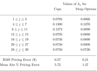
The root mean square pricing error for caps in Table 5 is greater than that for swap options. This reflects the fact that we are fitting the model to 133 caps and only 30 swap options. The relatively high average absolute percentage error for caps reflects both this and the existence of some errors in deep-out-of-the-money caps that, although small in absolute terms, were large when measured as percentages.
5.1 Incorporating Volatility Skews when European Swap Options are Priced As already mentioned broker quotes are available only for at-the-money European swap options. This is probably because, when they are initiated, most European swap options are close to the money. However, financial institutions are faced with the problem of marking to market their portfolios each day. Although they are usually close to the money when they first trade, European swap options are liable to be significantly in or out of the money when marked to market at a later date.
The analysis in Section 4 makes it possible to calculate a complete volatility skew for European swap options from broker quotes on at-the-money instruments. The procedure is as follows.
1. Calculate the price of the at-the-money swap option from its volatility using equation (10) or (11)
equation (33) or (35) with α set equal to its best fit value
3. Use this value of σn,N to calculate the price of non-at-the-money European swap
option using equation (33) or (35)
4. Imply a Black volatility for the non-at-the-money swap options using equation (10) or (11)10
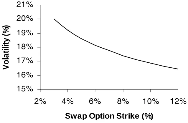
As an example we consider a 5×5 European swap option on August 12, 1999. (For the purposes of calculating the volatility skew it does not matter whether it is an option to receive fixed or receive floating.) The broker quote for the volatility of this instrument is 17.58% and the at-the-money strike swap rate is 7.47%. The results of the above procedure are displayed in Figure 3.
Note that the calculation of a volatility skew for European swap options depends only on the best fit value of α (0.716 for the case considered) and the at-the-money volatilities. It does not require an estimate of the Λj or the λj,q. It should be relatively easy for
financial institutions to store a value of α and update it periodically so that very fast volatility skew calculations can be made whenever required.
10 In theory, this last step is unnecessary since the third step provides the price. In
6. CONCLUSIONS
Caps and European swap options are quite different instruments. A cap is a portfolio of options; a European swap option is an option on an annuity. This paper has provided a simple robust procedure for relating the volatilities used by the market to price European swap options to the volatilities used by the market to price caps. Given the popularity of caps and European swap options, the procedure presents traders with opportunities to fine tune their pricing and search for arbitrage opportunities. A key contribution of the results in the paper is to make it very easy for traders to quickly calculate volatility skews for European swap options (which are not provided by brokers) from volatility skews for caps (which are provided by brokers).
REFERENCES
Andersen, L. A Simple Approach to the Pricing of Bermudan Swaptions in the Mul-tifactor LIBOR Market Model, Working paper, Gen Re Financial Products, 1998, forthcoming, Journal of Computational Finance.
Andersen L. and J. Andreasen, Volatility Skews and Extensions of the LIBOR Market Model, Working paper, Gen Re Financial Products, 1997, forthcoming, Applied
Mathematical Finance.
Black, F. The Pricing of Commodity Contracts,Journal of Financial Economics, 3 (March 1976), 16779.
Brace, A, D. Gararek, and M. Musiela. The Market Model of Interest Rate
Dynam-ics, Mathematical Finance, 7, 2 (1997), 12755.
Broadie, M. and P. Glasserman. A Stochastic Mesh Method for Pricing High Dimen-sional American Options, Working Paper, Columbia University, New York, 1997.
Harrison, J. M. and D. M. Kreps. Martingales and Arbitrage in Multiperiod Securi-ties Markets, Journal of Economic Theory, 20 (1979), 381408.
Heath, D., R. Jarrow, and A. Morton. Bond Pricing and the Term Structure of Interest Rates: A New Methodology, Econometrica, 60, 1 (1992), 77105.
Hull, J. C.Options, Futures, and Other Derivatives, Fourth Edition, Prentice Hall, Englewood Cliffs, NJ, 2000.
Jackwerth, J.C. and M. Rubinstein, Recovering Probability Distributions from Op-tion Prices, Journal of Finance, 51 (December 1996), 161131
Jamshidian, F. The LIBOR and Swap market Models, Finance and Stochastics, 1 (1997), 293330.
Longstaff, F. and E. Schwartz. Valuing American Options by Simulation: A Least Squares Approach, Working Paper 25-98, 1998, Andersen School at UCLA.
Miltersen, K., K. Sandmann, and D. Sondermann. Closed Form Solutions for Term Structure Derivatives with Lognormal Interest Rates, Journal of Finance, 52, 1 (March 1997), 40930.
Rebonato, R. On the Simultaneous Calibration of Multifactor Lognormal Interest rate Models to Black Volatilities and to the Correlation Matrix, Journal of
Table 1
Values of λj,q/Λj Used
The table shows values forλj,q/Λj, the ratio of the qth component of the volatility of a
forward rate to the total volatility of the forward rate. These were used to produce the results in Tables 3, 4, and 5.
Forward Rate Maturity (yrs)
q 1 2 3 4 5 6 7 8 9
Table 2
Accuracy of Caplet Volatilities
The table shows the amount by which the true spot caplet volatility exceeds the volatility given by the Monte Carlo implementation of the LIBOR market model in equation (22). For example, when the average rate is 1%, the average volatility is 50%, and the true caplet volatility is V%, the Monte Carlo simulation produces a price consistent with a volatility of V + 0.08%. The standard error of the volatility difference is in parentheses. Results are for 200,000 antithetic simulation trials, an upward sloping term structure, and a humped volatility structure. The caplet has a maturity of five years and tenor of one year. All volatilities are measured as percentages.
Average Average Volatility
Rate 10% 20% 50% 100%
1% 0.01 (0.02) 0.01 (0.05) 0.08 (0.25) 0.25 (1.19)
5% 0.02 (0.02) 0.02 (0.05) 0.56 (0.17) 2.57 (0.60)
10% 0.02 (0.02) 0.01 (0.04) 0.02 (0.12) 9.42 (0.44)
20% 0.01 (0.02) 0.02 (0.03) 0.39 (0.08) 14.64 (0.43)
Table 3
Accuracy of Swap Option Volatilities
The table shows the amount by which 5 × 5 swap option spot volatilities, calculated using the approximation in Section 3, exceed those calculated using the Monte Carlo implementation of the LIBOR market model in equation (22). For example, when the average rate is 1%, the average volatility is 50%, and the swap option volatility calculated from the approximation in section 3 is V%, the Monte Carlo simulation produces a price consistent with a volatility ofV −0.05%. The standard error of the Monte Carlo estimate is in parentheses. Results are for 200,000 antithetic simulation trials, an upward sloping term structure, and a humped volatility structure. Both the caps underlying the LIBOR market model and the swaps underlying the swap option are reset annually. All volatilities are measured as percentages.
Average Average Volatility
Rate 10% 20% 50% 100%
1% 0.01 (0.01) 0.02 (0.02) 0.05 (0.02) 1.00 (0.06)
5% 0.01 (0.01) 0.00 (0.02) 0.14 (0.04) 3.29 (0.05)
10% 0.00 (0.02) 0.02 (0.03) 0.34 (0.08) 5.11 (0.16)
20% 0.01 (0.02) 0.04 (0.04) 1.01 (0.14) 4.13 (0.35)
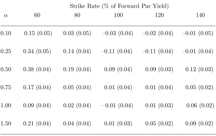
Table 4
Accuracy of Swap Option Volatilities When There is a Volatility Skew The table shows the amount by which 3×3 swap option volatilities calculated from the approximation in Section 4 exceed those calculated using the Monte Carlo implementation of the extended LIBOR market model in equation (27). For example, when α is 0.50, the strike rate is 80% of the forward par yield 1%, and the lognormal swap volatility calculated using Section 4 is V%, the Monte Carlo simulation produces a price consistent with a lognormal volatility of V −0.19%.The standard error of the Monte Carlo price is in parentheses. Results are for 100,000 antithetic simulation trials, an upward sloping term structure and a humped volatility structure. Caps used to define the LIBOR market model are reset quarterly and the swap underlying the swap option is reset semiannually. All volatilities are measured as percentages.
Strike Rate (% of Forward Par Yield)
α 60 80 100 120 140
0.10 0.15 (0.05) 0.03 (0.05) 0.03 (0.04) 0.02 (0.04) 0.01 (0.05)
0.25 0.34 (0.05) 0.14 (0.04) 0.11 (0.04) 0.11 (0.04) 0.01 (0.04)
0.50 0.38 (0.04) 0.19 (0.04) 0.09 (0.04) 0.09 (0.03) 0.12 (0.03)
0.75 0.17 (0.04) 0.05 (0.04) 0.01 (0.04) 0.01 (0.04) 0.05 (0.02)
1.00 0.09 (0.04) 0.02 (0.04) 0.01 (0.04) 0.01 (0.03) 0.06 (0.02)
Table 5
Best Fit Values of Volatility Parameters on August 12, 1999
The table show best fit values for the volatility parameters, Λj when the model defined
by equations (26) to (28) is fitted to 133 caps (column 2) and 30 European swap options (column 3). The CEV parameter α was set equal to its best fit value of 0.716. Princi-pal=$1,000 and δj = 0.25 for all j.
Values of Λj for
Caps Swap Options
1≤j ≤3 0.0795 0.0866
4≤j ≤7 0.1300 0.1076
8≤j ≤11 0.1274 0.0890
12≤j ≤15 0.0795 0.0890
16≤j ≤19 0.0756 0.0890
20≤j ≤27 0.0756 0.0808
28≤j ≤39 0.0756 0.0730
RMS Pricing Error ($) 0.57 0.21
(a) Swap Option 14% 16% 18% 20% 22% 24% 26%
60% 80% 100% 120% 140% Strike (% of par yield)
Im p li e d V o la ti li ty alpha=0.5 alpha=1 alpha=1.5 Cap 14% 16% 18% 20% 22% 24% 26%
60% 80% 100% 120% 140% Strike (% of Par Yield)
Im p li e d V o la ti li ty alpha=0.5 alpha=1 alpha=1.5 (b) Swap Option 14% 16% 18% 20% 22% 24% 26%
60% 80% 100% 120% 140% Strike (% of par yield)
Im p li e d V o la ti li ty alpha=0.5 alpha=1 alpha=1.5 Cap 14% 16% 18% 20% 22% 24% 26%
60% 80% 100% 120% 140% Strike (% of Par Yield)
[image:38.612.158.498.170.408.2]Im p li e d V o la ti li ty alpha=0.5 alpha=1 alpha=1.5 Figure 1
(a) Swap Option 14% 16% 18% 20% 22% 24% 26%
60% 80% 100% 120% 140% Strike (% of par yield)
Im p li e d V o la ti li ty alpha=0.5 alpha=1 alpha=1.5 Cap 14% 16% 18% 20% 22% 24% 26%
60% 80% 100% 120% 140% Strike (% of Par Yield)
Im p li e d V o la ti li ty alpha=0.5 alpha=1 alpha=1.5 (b) Swap Option 14% 16% 18% 20% 22% 24% 26%
60% 80% 100% 120% 140% Strike (% of par yield)
Im p li e d V o la ti li ty alpha=0.5 alpha=1 alpha=1.5 Cap 14% 16% 18% 20% 22% 24% 26%
60% 80% 100% 120% 140% Strike (% of Par Yield)
[image:39.612.158.497.177.418.2]Im p li e d V o la ti li ty alpha=0.5 alpha=1 alpha=1.5 Figure 2
15%
16%
17%
18%
19%
20%
21%
2%
4%
6%
8%
10%
12%
Swap Option Strike (%)
V
o
la
ti
lit
y
(%
)
[image:40.612.149.468.226.435.2]Figure 3