Estimation of the Libor Market Model:
Combining Term Structure Data and Option
Prices
Frank De Jong
Joost Driessen
Antoon Pelsser
This version: February, 2001
Frank de Jong, Finance Group, University of Amsterdam, Roetersstraat 11, 1018 WB, Amsterdam, The Netherlands. Tel: +31-20-5255815. E-mail: [email protected].
Joost Driessen, Department of Econometrics, Tilburg University, PO Box 90153, 5000 LE, Tilburg, The Netherlands. Tel: +31-13-4663219. E-mail: [email protected].
Estimation of the Libor Market Model:
Combining Term Structure Data and Option
Prices
Abstract
Previous empirical work on term structure models has estimated and tested these models on the basis of either interest rate data or derivative price data. In this paper, we analyze the benefits of combining these two data sets for estimating and testing multi-factor Libor market models. We use US data on interest rates and prices of caps and swaptions from 1995 to 1999. We allow for the presence of measurement error in both the interest rates and the option prices. The results on the fit of a two-factor model show that, in case of estimation based on option prices only, the model does not accurately fit the standard deviations of interest rate changes, and, in case of estimation on the basis of interest rate data, the model misprices caps and, especially, swaptions. Thus, the two-factor model cannot fit the main features of the two data sets at the same time. This result illustrates the benefit of using both interest rate data and option price data for testing term structure models. A three-factor model provides a much better fit to both the interest rate data and the option price data. In particular, the humped shape of the volatility term structure is fitted more accurately.
JEL Codes: G12, G13, E43.
1 Introduction
Previous empirical work on term structure models has estimated and tested these models on the
basis of interest rate data (for example, Buhler et al. (1999), Dai and Singleton (2000), De Jong
(2000), Pearson and Sun (1994)), or derivative price data (Amin and Morton (1994), Flesaker
(1993)). There are several potential benefits of combining these two data sets to estimate and test
term structure models. First, model parameters might be estimated more precisely. In particular,
for estimating multi-factor term structure models (that have a large number of parameters) using
both interest rate data and option prices seems beneficial. Second, using both data sets to test
term structure models will likely give stronger tests of these models. For example, it might be the
case that a given model provides a reasonable fit of the main features of interest rate data, but
considerably misprices interest rate options. Therefore, in this paper, we estimate and test
multi-factor term structure models using both interest rate data and option price data, and investigate
the benefits of using both data sets.
The models that we analyze are in the class of the Libor Market Models (Brace, Gatarek, and
Musiela (1997), Miltersen, Sandmann, and Sondermann (1997), and Jamshidian (1997)). We
specify a multi-factor Libor Market Model with correlated factors, where each factor has a
time-homogeneous volatility function that corresponds to mean-reverting behaviour of the factor. This
way, the model is related to the affine class of term structure models (Duffie and Kan (1996)),
and, in particular, to the stochastic mean model of Jegadeesh and Pennacchi (1996). In the latter
model, the short rate is mean reverting around a ‘shadow’ rate, that itself is (slowly) mean
reverting around a constant mean. By allowing the factors to be correlated, the model is able to
generate a humped shape for the term structure of interest rate volatilities.
For the empirical analysis, we use weekly US data on Libor and swap rates and prices for
caps and swaptions from 1995 to 1999. The model setup explicitly allows for the presence of
measurement error in both the interest rates and derivative prices. Given this model setup,
moment restrictions are derived for both variances and covariances of changes in forward Libor
interest rates of different forward maturities, and for the expected prices of several caps and
swaptions. Estimation is performed by applying the Generalized Method of Moments (GMM,
Hansen (1982)). We estimate both two-factor and three-factor models, thereby extending the
analyzed. For comparison, we also estimate the models both only on the basis of interest rate data
and only on the basis of option price data.
First, we analyze whether using both interest rate and option price data leads to more
accurate parameter estimates. For both the two-factor and three-factor model, we find that, when
estimating the model using both interest rate and option price data, the standard errors of the
parameter estimates are not always smaller than the standard errors that result when only interest
rate data or option price data are used for estimation.
Second, we analyze the fit of the models on the interest rate and option price data. The results
for the two-factor model show that, in case of estimation based on option prices only, the model
does not accurately fit the standard deviations of forward Libor rate changes, and, in case of
estimation on the basis of interest rate data, the model misprices caps and, especially, swaptions.
Thus, the two-factor model cannot fit the main features of the two data sets at the same time.
This result illustrates the benefit of using both interest rate data and option price data to test term
structure models. In case of joint estimation, there is a trade off between the fit on the option
price data and the fit on the interest rate data, but the two-factor model still poorly fits both the
forward Libor rate (co)variance structure and the maturity patterns in the cap and swaption
prices. In particular, the model is not capable of both fitting the humped shape of the term
structure of interest rate volatilities and the cross-correlations between forward Libor rate
changes.
The three-factor model provides a better fit to both the interest rate data and the option price
data. Both the humped shape of the standard deviations of forward Libor rate changes, and the
humped shape of the cap implied volatility curve are fitted more accurately. Still, the model
slightly overprices swaptions, and the model implies correlations between forward Libor rate
changes that are a bit lower than in the data.
In line with results of Dai and Singleton (2000) and De Jong (2000), we find that the
correlations between the factors are significantly different from zero. These nonzero correlations
are necessary to generate a hump shaped volatility curve. The results also show that allowing for
measurement error in the interest rates is an important aspect of the model setup. Neglecting this
measurement error structure would lead to overpricing of caps and too low standard deviations
of forward Libor rate changes. However, for all models the estimate for the variance of the Libor
on the measurement error structure.
The remainder of this paper is organized as follows. Section 2 discusses and motivates the
modeling framework. Section 3 describes the interest rate data and option price data, as well as
the estimation methodology. Section 4 contains the estimation results for two-factor and
three-factor models. Section 5 concludes.
2 Modeling Framework
2.1 Libor Market Model
To jointly analyze both term structure data and option price data, we choose the Libor Market
Model (LMM) as modeling framework. The reason for using the LMM is threefold. First of all,
the LMM is often used by financial institutions. Second, our option price data consist of implied
Black (1976) volatility quotes for caps and swaptions, and the LMM implies simple Black-type
pricing formulas for caps (and approximate pricing formulas for swaptions), which facilitates the
estimation of the model. Third, De Jong, Driessen, and Pelsser (2000) provide evidence that the
LMM outperforms the Swap Market Model (SMM) in pricing caps and swaptions. In De Jong,
Driessen, and Pelsser (2000) other advantages of the market models are mentioned.
We describe the LMM formulation based on a finite number of bond prices, following
Jamshidian (1997). We start with defining a finite set of dates T1 < T2 < ... < TN, the so-called
tenor structure. We also define *i ' T as the so-called daycount fractions,
i%1&Ti, i'1,..,N&1
which are determined by the maturity of the Libor rate that is used to determine caplet payoffs
and are most often equal to 3 or 6 months. Associated with each tenor date Tn is a bond that matures at this date, and its time t price is denoted with Pn(t). These N bond prices, with maturities T1,...,TN, determine (N-1) forward Libor rates.
We analyze a multi-factor LMM with K factors. This multi-factor LMM implies that the forward Libor rate Ln(t), defined by Ln(t) ' 1 , satisfies the following Itô process
*n(
Pn(t)
Pn%1(t)
&1)
dLn(t) ' Ln(t) (& j
N&1
i'n%1
*iLi(t)(i(t))E(n(t) 1%*
iLi(t)
dt % (n(t))dW((t) ), n'1,...,N&1 (2)
dLn(t) ' L
n(t) µn(t)dt % Ln(t)(n(t)
)
dW(t) , n'1,...,N&1 (1)
The function µn(t) is the drift function of the forward Libor rate, and(n(t) is a, deterministic, K -dimensional vector that is often referred to as the volatility function. W(t) is a K-dimensional vector of correlated Brownian motions. The correlation between the ith component and jth
component of W(t) is denoted by Dij. By choosing one of the N bonds as the numeraire asset, we can obtain the process of the forward Libor rates under the equivalent martingale measure
associated with this numeraire choice. Under such an equivalent martingale measure, the drift of
the forward Libor rates is completely determined by the volatility functions (n(t), n=1,..,N-1, see Jamshidian (1997). For example, if we take the longest maturity bond PN(t) as the numeraire, we obtain the so-called terminal measure QN, under which forward Libor rates follow the process
where W((t) is a K-dimensional Brownian motion under the terminal measure, and where isE the instantaneous correlation matrix of this Brownian motion, so that is a E K by K matrix with the (i,j)th component equal to D .
ij
Equation (2) implies that, in order to price and hedge interest rate derivatives, only the
volatility functions (n(t) have to be determined. We refer to Brace, Gatarek, and Musiela (1997) and Jamshidian (1997) for the pricing formulas for caps and swaptions. Most importantly, these
formulas show that, in the LMM, cap prices depend on conditional variances of forward Libor
rates, whereas swaption prices both depend on conditional variances of forward Libor rates, and
conditional covariances between forward Libor rates of different maturities.
2.2 Specification of Volatility Functions
1
The instantaneous covariance matrix of the Brownian motions has to be symmetric and positive definite. These restrictions are imposed when estimating the model parameters.
2
f(t,T) is the time t forward rate for instantaneous lending at time T.
dXi(t) ' &6iXi(t)dt % FidZi(t) (4)
df(t,T) ' drift dt % j
K
i'1
Fiexp(&6
i(T&t))dZi(t) (5)
(n(t) ' (F
1exp(&61(Tn&t)),....,FKexp(&6K(Tn&t)))
)
, n'1,...,N&1 (3)
function can lead to overfitting to option prices, and also provide empirical evidence in favour
of a declining volatility function instead of a constant volatility function. Furthermore, Dai and
Singleton (2000) illustrate that allowing for nonzero correlations between factors in (affine) term
structure models is important for accurately describing US interest rate behaviour. Therefore, we
choose the following time-homogeneous specification for the volatility functions in the LMM
and allow for an unrestricted correlation matrix G for the Brownian motions1. In the remainder, we will refer to the parameter Fi as the volatility parameter of factor i and to the parameter 6i as its decay parameter.
These volatility functions are very similar to the volatility functions implied by the affine term
structure models of Duffie and Kan (1996). In particular, consider a K-factor version of the Vasicek (1977) model. In this model, the instantaneous short rate r(t) is the sum of a constant and K factors, i.e., r(t) ' 2 % jK , where each factor follows a mean reverting process
i'1 Xi(t)
under the true probability measure with parameter 6i, that determines the strength of the mean
reversion, and volatility parameter Fi
The vector of Brownian motions Z(t) ' (Z1(t),...,ZK(t))) is assumed to have instantaneous correlation matrix . It is easy to show that, if the factor risk prices are deterministic, this modelE
3
This follows from choosing X1(t) ' (r(t)&2) & (2(t)&2)a/(a&b) and X .
2(t) ' (2(t)&2)a/(a&b)
dr(t) ' a(2(t) & r(t))dt % F
rdZ r(t)
d2(t) ' b(2 & 2(t))dt % F
2dZ2(t)
Cov(dZr(t),dZ2(t) ) ' D
r2FrF2dt
(6) under the true probability measure. Under the equivalent martingale measure, the diffusion terms
in equation (5) remain unchanged and only the drift changes. Equation (5) shows that, in the K -factor Vasicek model, changes in instantaneous forward rates are determined by K correlated factors with volatility functions Fiexp(&6 . Because the factor is strictly mean reverting,
i(T&t))
this volatility function is decreasing in the time to maturity (T-t). The parameter 6i determines the decay in the volatility function: strong mean reversion for a factor implies that the volatility
function declines quickly.
Equation (3) shows that we choose the same volatility functions for the LMM, which then
apply to the changes in log forward Libor rates instead of instantaneous forward rates. This
choice facilitates the interpretation of the decay parameter 6i: it is linked to the mean reversion
of factor i.
In case of a two-factor model, the Vasicek instantaneous spot rate model has a particularly
interesting interpretation, since this model can be rewritten as3
This is the central tendency model of Jegadeesh and Pennacchi (1996). In such a central tendency
model the short rate is mean reverting around a ‘shadow rate’ (the central tendency). This
shadow rate itself is mean reverting around a constant mean. Jegadeesh and Pennacchi claim that
this model is much more adequate in describing the dynamics of Eurodollar futures prices than
a one-factor model. Also, Jegadeesh and Pennacchi show that the central tendency model is able
to generate a humped structure for forward Libor rate volatilities, which is a feature of the US
Libor rate data and the cap data that we analyze. One can show that, to generate a humped
3 Data and Estimation Method
3.1 Data
We use two data sets: one data set containing US money-market rates and swap rates and
another data set containing implied Black (1976) volatilities of US caps and swaptions. For both
data sets we have 232 weekly observations from January 1995 until June 1999.
We use the US money-market rates with maturities of 1, 3, 6, 9, and 12 months, and the data
on US swap rates with maturities ranging from 2 to 15 years to estimate the instantaneous
forward rate curve using an exponential splines specification. This way, we obtain a trade off
between fit of the money-market and swap rates and smoothness of the forward rate curve. Since
estimates for forward (Libor) rates are very sensitive to small differences between money market
or swap rates of nearly the same maturity, a perfect fit of all underlying money market and swap
rates generally leads to unrealistically high estimates for the standard deviations of historical
forward (Libor) rate changes, and low correlations between these forward Libor rates. Therefore,
we impose some smoothness conditions on the shape of the forward interest rate curve via the
exponential splines specification. This gives us at each week instantaneous forward rates f(t,T), from which we construct forward Libor rates for different forward maturities and 3-month Libor
maturity. In Table 1 we give the correlation matrix of weekly changes in the logarithm of these
forward Libor rates and in Figure 1 the annualized standard deviations of these changes are
plotted. In line with results presented in Amin and Morton (1994), and Moraleda and Vorst
(1997), Figure 1 shows that there is evidence for a humped volatility structure for forward Libor
rate changes.
The derivatives data that we use are weekly quotes for the implied Black (1976) volatilities
of at-the-money-forward US caps and swaptions, in total 63 instruments. The caps have
maturities ranging from 1 to 10 years, and their payoffs are defined on 3-month Libor rates. The
1-year cap consists of 3 caplets with maturities of 3, 6, and 9 months, and the 10-year cap
consists of 39 caplets, with maturities ranging from 3 months to 9 years and 9 months. The other
caps are constructed in a similar way. The strike of each cap is equal to the corresponding swap
Cov(dlnLi(t),dlnLj(t)) ' (
i(t)
)E(
j(t)dt, i,j'1,...,N&1 (7)
volatilities of the caps. Again there is evidence for a hump shaped volatility structure.
For the swaptions, the option maturities range from 1 month to 5 years, while the swap
maturities range from 1 to 10 years. The strike of an at-the-money swaption is equal to the
corresponding forward swap rate. These data again provide evidence for a hump shaped volatility
structure.
3.2 Estimation Methodology
In this paper, we focus on estimating the diffusion parameters or volatility functions of the
forward Libor rate processes. To estimate these parameters, we derive moment restrictions that
can be applied to the forward Libor rate data and the cap and swaption price data, and use the
Generalized Method of Moments to estimate the models. We use two sets of moment
restrictions:
1. Variances of log forward Libor rate changes and covariances between log forward Libor rate
changes of different forward maturities.
2. Expected cap implied volatilities and swaption implied volatilities.
We refer to estimation on the basis of the first set of moments as interest-rate-based estimation, and to estimation on the basis of the second set of moments as option-based estimation. The use of both sets of moment restrictions is referred to as joint estimation. All moment restrictions are formulated under the true probability measure.
The first set of moment restrictions is based on the fact that the LMM implies that (under the
4
This approximate relation is only exact if the drift of the log forward Libor rates is deterministic, which is in general not the case. If the market prices of interest rate risk are very volatile or if the mean reversion parameter is extremely large, the approximation error might be important.
lnLi((t) ' lnL
i(t) % ,i(t), E(,i(t)) ' 0, i'1,..,N&1 (8)
V(,i(t)) ' F2,, Cov(,
i(t),,j(t)) ' 0, i,j'1,...,N&1, i…j (9)
By approximation, this relation holds for small time intervals )t.4 The use of variances and
covariances for estimation can be motivated by the fact that, if we neglect the drift of Libor rates,
the (conditional) distribution of log forward Libor rates is normal. In line with previous research
on term structure models (for example, De Jong (2000), Duan and Simonato (1999), Duffee
(1999)), we assume that the log forward Libor rate that we observe, lnLi((t), is equal to the true log forward Libor rate lnLi(t), plus a zero-expectation error term ,i(t), that is independently and identically distributed over time and forward maturities, and independent of the true log forward
Libor rate lnLi(t):
For simplicity, we assume that the error terms are maturity-specific and that the error variance
is constant over forward maturities
There are several reasons to include the error term in the log forward Libor rate. First of all, the
forward Libor rates are estimated using the exponential splines specification, which might induce
some estimation error in the forward Libor rate estimates. Second, the underlying money-market
and swap data might contain measurement error due to illiquidity and time-of-the-day effects.
Third, the weekly first-order autocorrelation in the log-forward Libor rate changes is, averaged
over all forward maturities, equal to -0.185, whereas the higher-order autocorrelations are close
to zero or even positive. This supports the model, since it is easy to show that, abstracting from
the drift of forward Libor rates that is implied by the model, (1) and (8) lead to negative
first-order autocorrelation for discrete-time changes in the forward Libor rate, and zero
5
To perform GMM on variance and covariance restrictions, we add auxiliary moment restrictions of the form , where the `s are free coefficients that are estimated along with the other
E()lnLi((t) ) ' "
i, i'1,...,N&1 "i
parameters. Even if the true means (i.e., the "i`s) are equal to zero, which would be the case if forward Libor rates are stationary, Cochrane (2001) notes that, in small samples, better estimates are obtained if one uses variances and covariances instead of second moments. In our case, the sample means are very small relative to the variance of the forward Libor rates, so that imposing that the "i`s are equal to zero hardly affects the GMM parameter estimates.
6
The assumption that this error term has zero expectation should be interpreted as an approximate moment restriction, due to the dependence of the LMM Black volatility IVC,LMM(t,T on the underlying forward Libor
i)
rates. If this dependence would be linear, the presence of measurement error in the forward Libor rates would not change the unconditional expectation of IVC,LMM(t,Ti). In reality, this dependence is, however, not linear, so that the expectation of IVC,LMM(t,T will depend on the variance of the measurement error in the forward Libor rates
i)
(and higher-order moments of the measurement error distribution). A Taylor expansion shows that, for at-the-money-forward caps and swaptions, this is a second order effect, and we will therefore neglect this effect in estimating the model.
V()lnLi((t)) ' (
i(t)
)E (
i(t))t % 2F
2
,, i'1,...,N&1
Cov()lnLi((t),)lnLj((t)) ' (
i(t)
)E (
j(t))t, i,j'1,...,N&1
(10) Note that the measurement error assumption in (8) changes the variance of the forward Libor
rate changes, whereas it leaves the covariances between forward Libor rates unchanged. This
way, the first set of moment restrictions is given by5
In Section 5.4.1 similar moment restrictions are formulated for changes in instantaneous forward
rates and HJM models, but without the measurement error variance. Using data on the log
forward Libor rates, we can estimate the right hand sides of equation (10) and confront these
estimates with the model-implied (co)variances. For estimation, we annualize the (co)variances
by multiplying (10) with 1/)t such as to obtain the same scaling for these restrictions as the implied volatilities (see below).
To derive the moment restrictions for derivative prices, we assume that the (square of the)
observed implied Black volatility quote for a cap or swaption is equal to the (square of the) Black
implied volatility that corresponds to the model price, plus an independent zero-expectation error
term,6 that represents measurement error in the observed implied volatility quote. For caps, we
7
This expectation is taken under the true probability measure, since the option prices are observed under this measure. Of course, to calculate the option prices implied by the LMM, one uses an equivalent martingale measure.
[IVC(t,Ti)]2 ' [IVC,LMM(t,T i))]
2 % 0
i(t), E(0i(t)) ' 0 (11)
where IVC(t,T is the observed implied volatility for the cap with maturity Ti, and where
i)
is the implied volatility for this cap that corresponds to the cap price implied by
IVC,LMM(t,Ti)
the LMM. A similar expression results for swaptions. We take the square of the implied
volatilities so that these moment restrictions are measured with the same scale as the restrictions
in (7). By taking the expectation on both sides of equation (11) we obtain moment restrictions
for caps and swaptions7.
By approximation, the measurement error variance of the forward Libor rates does not enter
the moment restrictions for caps and swaptions. Thus, by combining the forward Libor rate
moment restrictions and the cap and swaption restrictions, the measurement error variance can
be estimated precisely. Because the measurement error variance does not enter the cap and
swaption moment restrictions, this measurement error variance cannot be estimated in case of
option-based estimation. In this case, given the option-based parameter estimates, the
measurement error variance is estimated from the forward Libor variance moment restrictions.
As noted above, in the LMM, the prices of caps depend on the conditional variances of Libor
rates, whereas the prices of swaptions depend both on conditional variances of forward Libor
rates, and on the conditional covariances between forward Libor rates of different forward
maturities. Thus, both sets of moment restrictions involve (conditional) variances and covariances
of forward Libor rates, and from both sets of moment restrictions it is possible to identify the
parameters of models with multiple factors.
We use the Generalized Method of Moments (Hansen (1982)) to estimate the parameters of
two- and three-factor LMMs. We select some forward maturities and option maturities for the
moment restrictions, to obtain roughly the same number of moment restrictions for
interest-rate-based estimation and option-interest-rate-based estimation. For the forward Libor rate variance restrictions,
we choose the following forward maturities (in years): 0.25, 0.75, 1.25, 1.75, 2.75, 3.75, 4.75,
8
We use the method of Newey and West (1987) to correct this covariance matrix for heteroskedasticity and autocorrelation.
For the covariance restrictions, we take the covariances between forward Libor rate changes with
forward maturities of 0.25 years, 1.25 years, 2.75 years, 4.75 years, and 9.75 years, in total 10
moment restrictions.
For the cap moment restrictions, we use all 7 option maturities that are available in the cap
data, ranging from the 1-year cap to the 10-year cap. Since there are 56 different swaptions in
the data set, we select a subset of these swaptions. We choose three option maturities, 3 months,
1 year, and 5 years, and three swap maturities, 1 year, 3 years, and 5 years. Taking all
combinations gives us 9 moment restrictions for the swaptions.
In the first step of GMM, we choose an identity weighting matrix. Recall that we formulated
all moment restrictions such that they all refer to annualized variances and covariances, so that
giving equal weights to all moment restrictions is not unreasonable. Also, the number of moment
restrictions is roughly the same for the Libor variances, Libor covariances, cap volatilities, and
swaption volatilities, so that none of these four sets of restrictions dominates the first-step
estimation results.
It turns out that the covariance matrix of these estimated moment restrictions is close to
singularity8. In other words, the estimated moment restrictions are highly correlated (especially
the restrictions for the caps and swaptions). The efficient, second step of GMM requires that the
inverse of the covariance matrix of the estimated moment restrictions is used as the weighting
matrix. As shown by Hansen (1982), this is the optimal choice for a correctly specified model in
the sense that it yields the lowest asymptotic variance for the GMM parameter estimates.
However, as noted by Cochrane (2001), if the covariance matrix of the moment restrictions is
close to singularity, using this covariance matrix as weighting matrix implies that one fits the
model parameters to linear combinations of the original moment restrictions that have very large
positive and negative weights on the original moment restrictions. Using these linear
combinations of moment restrictions to estimate the model might be statistically optimal for a
correctly specified model (that is, asymptotically), but one can question whether these extreme
linear combinations are the most interesting moment restrictions from an economic point of view
(see Cochrane (2001)). Focusing on these extreme linear combinations might, therefore,
9
To see this in a simple example, suppose one fits a one-parameter model to the 1-year and 2-year forward Libor variances. These Libor variance estimates are highly positively correlated. If one performs a Cholesky decomposition of the optimal weighting matrix (the inverse of the covariance matrix), one finds that the second-step GMM estimates are obtained by fitting to the 1-year forward Libor variance, and to the difference between the 2-year and 1-year forward Libor variances, where this second moment restriction has a much higher weight than the first moment restriction.
10
For a given moment restriction, this t-ratio is defined by the ratio of the model error for this moment restriction and the standard error of this model error. This standard error is calculated using the asymptotic We find that, when using the optimal weighting matrix, the model is essentially fitted to the
differences between the moment restrictions rather than to the level of the moment restrictions,
since, due to the high correlations between the estimated moment restrictions, the standard errors
of these differences are much lower than the standard errors of the levels9. When performing
two-stage GMM estimation for our two-factor and three-factor models, we find that the shape
of the Libor variance term structure, the Libor covariance structure, and the cap and swaption
implied volatility term structures are fitted quite accurately, whereas the level of these term
structures is not fitted well. Therefore, we use in the empirical analysis in the next section only
the first-stage GMM estimator, that is obtained using an identity weighting matrix. Of course,
if the model is correctly specified, this estimator is still consistent and asymptotically normal, and
standard errors and tests are constructed in a straightforward way. In subsequent research, we
will analyze to what extent the differences between the first-stage and second-stage GMM
estimates are due to misspecification of the model and, in particular, to the restrictive
specification of the measurement error structure.
An alternative explanation for the current findings is that transaction costs for the options are
ignored. Driessen, Melenberg, and Nijman (1999) show that, without transaction costs, portfolios
with large short and long positions in near-maturity bonds are mispriced and lead to the rejection
of standard term structure models. If transaction costs are included, these portfolios are no longer
mispriced. One might expect a similar result here, now applied to positions in near-maturity
interest rate options instead of bonds. For simplicity, we do not explicitly include transaction
costs in this paper and use only first-stage GMM.
The near-singular covariance matrix of the moment restrictions also causes the GMM
J-statistic, that can be used to jointly test the overidentifying restrictions, to be very large for all
covariance matrix of the estimated moment restrictions (see also Gourieroux and Monfort (1995)).
11
In case of interest-rate based estimation, this correlation parameter is estimated at the lower bound of -0.999. In this case, for the calculation of standard errors and tests of moment restrictions the correlation parameter is treated as a constant.
restrictions to analyze the statistical accuracy of the models.
4 Empirical Results
There is much empirical evidence against one-factor term structure models. Also, given our
specification for the volatility functions in equation (3), it directly follows that one-factor models
cannot generate a humped volatility structure. Therefore, we focus on a two-factor and
three-factor model. As explained in the previous section, we will estimate both models three
times: on the basis of interest-rate-based estimation, option-based estimation, and joint
estimation.
4.1 Two-Factor Results
In this subsection we focus on the two-factor results. In Table 2, we give the parameter
estimates. First of all, we note that joint estimation does not always give more accurate parameter
estimates than interest-rate-based and option-based estimation. For all three estimation
methodologies, we find that the first factor has a relatively low decay parameter, whereas the
second factor has a high decay parameter. This implies that only forward Libor rates with very
short forward maturities are influenced by the second factor, and that the other forward Libor
rates are driven by the first factor only, which causes these forward Libor rates to be (almost)
perfectly correlated. The estimate for the correlation between the two factors is negative and
close to -111. This large negative correlation is needed to generate a humped volatility structure
for forward Libor rates and cap implied volatilities.
In case of option-based estimation, the volatility parameters and the decay parameters are
we thus find a stronger decay in the volatilities as function of maturity than based on
interest-rated based estimation.
Irrespective of the estimation methodology that is used, we find a large estimate for the Libor
measurement error standard deviation. For example, in case of joint estimation, this measurement
error standard deviation is estimated at 0.0088, implying that the forward Libor rates are
measured with an error that has a standard deviation roughly equal to 88 basis points. Thus, the
model implies that forward Libor rates are measured very imprecisely, and, although we argued
in Section 2 that it is likely that there is some measurement error in the forward Libor rates, this
amount of measurement error seems to be too large. This large estimate for the Libor
measurement error variance either implies that the term structure model is misspecified, or that
the assumptions on the measurement error structure are incorrect. For example, we have assumed
constant variance of the measurement error across forward Libor maturities, and no correlation
between measurement errors of different forward Libor rates. In future research we plan to
examine whether other measurement error assumptions lead to more reasonable estimates for the
size of the measurement error. In particular, one could argue that forward Libor rates with long
forward maturities are measured with higher error, since these rates are more sensitive to
measurement error in the underlying swap rate data.
For the three sets of parameter estimates for the two-factor model, the fit on the standard
deviations of forward Libor rates is shown in Figure 1. The figure shows that, although all
parameter estimates generate a humped standard deviation structure, the shape of the
model-implied standard deviation structure is clearly different from the standard deviation term
structure observed in the data. Also, the shape of the Libor standard deviation structure implied
by option-based estimation is different from the shapes implied by the other two estimation
methods: for long forward maturities, option-based estimation leads to lower forward Libor
standard deviations. Note also that, if we would not include the Libor measurement error in the
model, the option-based estimates would imply forward Libor standard deviations that are all
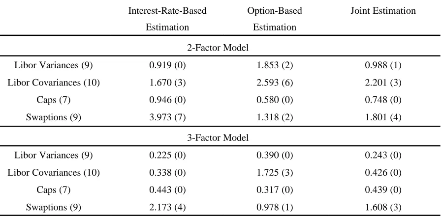
much lower than the observed standard deviations. Table 3 gives the average absolute t-ratios
for the individual moment restrictions. In case of interest-rate-based estimation, none of the Libor
variance moment restrictions is misfitted significantly by the model. In case of option-based
estimation, two out of the nine Libor variance moment restrictions are significantly misfitted by
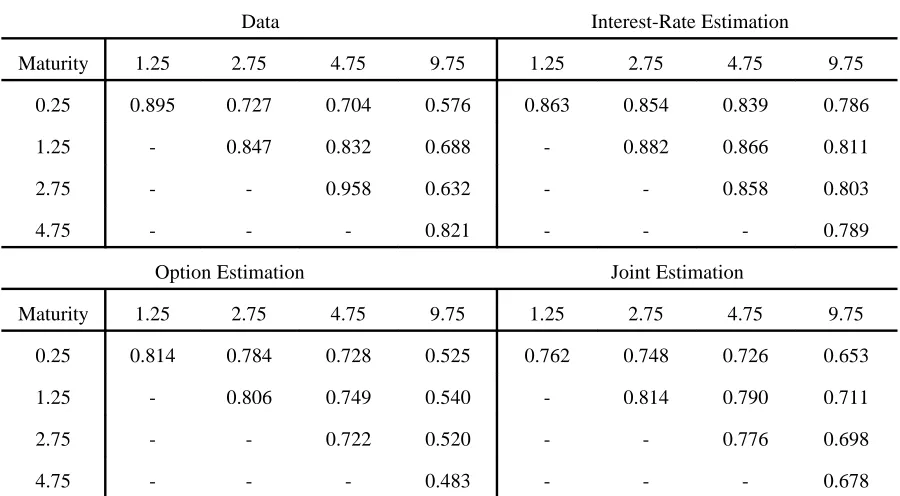
Table 1 gives the implications of the two-factor model for the cross-correlations of forward
Libor rates. As mentioned above, all three sets of parameter estimates imply that the two-factor
model itself yields almost perfect correlation between forward Libor rate changes of different
maturities. However, the presence of the forward Libor measurement error term generates some
decorrelation between forward Libor rates of different maturities. Since the Libor measurement
error variance is largest in case of option-based estimation, these parameter estimates lead to the
lowest correlations between Libor rates. However, Table 1 shows that none of the three sets of
parameter estimates leads to a very good fit of the correlation structure. In the data, the
correlation between forward Libor rates decreases when the difference between the two forward
maturities increases, and all three two-factor models do not always imply such a correlation
structure. This is confirmed by the t-ratios of the covariance moment restrictions in Table 3, that
show that at least three of the ten covariance moment restrictions are rejected by all three
two-factor models.
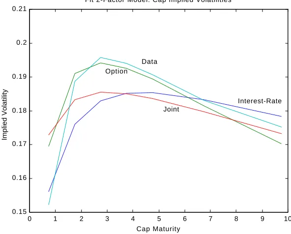
Figure 2 depicts the observed implied volatility term structure for caps, and the cap volatility
structures implied by the two-factor model. Of course, the option-based parameter estimates lead
to the best fit of these cap volatilities. Both interest-rate based estimation and joint estimation
lead to cap volatility structures that are too flat. Comparing these results with the forward Libor
standard deviations shows that the decay in the cap volatility term structure is larger than the
decay in the term structure of forward Libor rate standard deviations. Still, due to the large
variation and the large autocorrelation in cap implied volatilities over time, none of the models
imply significant mispricing of the caps.
Finally, in Figure 3 we plot the fit of the two-factor models on the swaption implied
volatilities. First of all, the figure shows that interest-rate-based estimation leads to too high
prices for swaptions, and Table 3 shows that the pricing errors are mostly statistically significant.
Still, the shape of the swaption volatility term structure that is implied by the interest-rate based
estimates is very similar to the observed shape. In case of option-based estimation, the two-factor
model gives a better fit of the level of swaption volatilities, but it does not accurately fit the shape
of the swaption volatility term structure: option-based estimation leads to swaption volatility term
structures that are too humped and that decline too much for longer maturities. Table 3 also
shows that, even in case of option-based estimation, some swaptions are still significantly
than the fit in case of option-based estimation and better than the fit in case of interest-rate based
estimation. In general, the two-factor model is not able to fit both the cap volatility structure,
which exhibits a strong hump and is declining for long maturities, and the swaption volatility
structure, which has only a small hump.
Summarizing, the two-factor model does not give a satisfactory fit of the data. First of all,
there are some inconsistencies between estimation based on interest-rate data and estimation on
the basis of option price data. In case of option-based estimation, the model does not accurately
fit the standard deviations of forward Libor rate changes. In case of interest-rate based
estimation, the model does not give a good fit of caps and, especially, swaptions. Second, even
in case of joint estimation, Table 3 shows that there are still some Libor (co)variances and option
prices that are significantly misfitted by the model. In particular, the two-factor model misfits the
correlation structure of forward Libor rates. The reason for this is the following. To generate a
humped volatility structure, the two factors need to be very highly negatively correlated, and one
factor needs to have a very high decay parameter. This implies that this factor only influences
very short maturity forward Libor rates, so that most forward Libor rates are essentially driven
by only one factor. The two-factor model thus implies almost perfectly correlated forward Libor
rates. Only due to the presence of the forward Libor measurement error structure, the model
generates some decorrelation between forward Libor rates, but the model-implied correlation
structure is quite different from the observed correlation structure. Therefore, in the next
subsection we analyze three-factor models.
4.2 Three-Factor Results
Table 4 presents the parameter estimates for the three-factor model for the three sets of moment
conditions. Again, joint estimation does not always give more accurate parameter estimates than
interest-rate-based and option-based estimation. For the three estimation methods, the estimates
for the volatility and decay parameters are quite similar to each other. One factor has a high
decay parameter, implying a quickly declining volatility function, another factor has a very low
decay parameter, implying a flat volatility function, and the third factor has an intermediate decay
parameter. Using interest rate data only and different estimation methods, Dai and Singleton
correlations between the factors that follow from option-based estimation are somewhat different
from the factor-correlations implied by interest-rate-based estimation and joint estimation. Below,
we discuss the implications of this difference. Finally, the Libor rate measurement error standard
deviation is around 70 basis points for all three estimation methods, which is roughly the same
as in the two-factor model. Therefore, adding a third factor does not ‘solve’ the problem of the
(too) large estimate for the Libor measurement error variance.
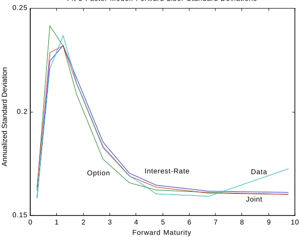
Figure 4 shows that all three estimation strategies provide a reasonable fit of the standard
deviations of forward Libor rates, and Table 3 shows that none of the forward Libor standard
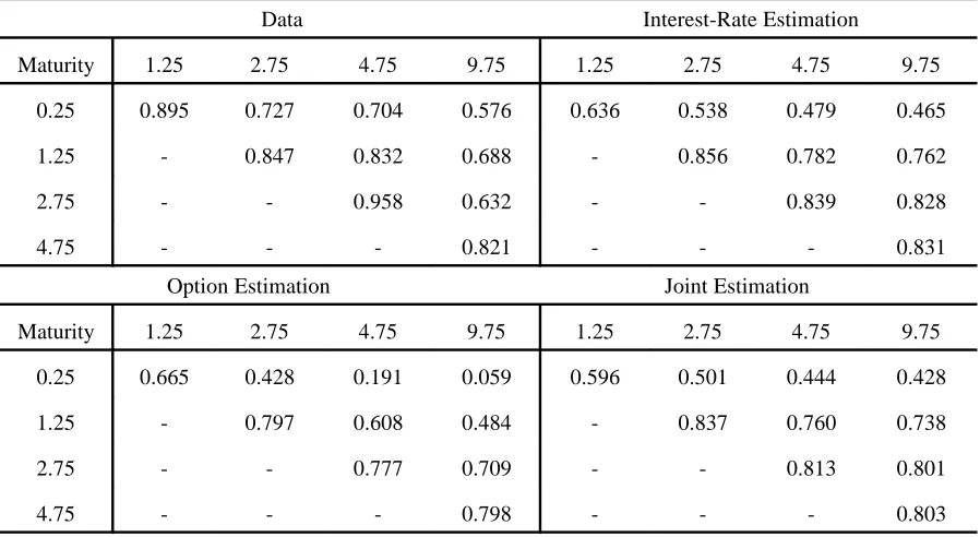
deviations is misfitted significantly. Table 5 gives the forward Libor correlation structures implied
by the three estimation strategies. Clearly, the fit is much better than in case of the two-factor
model, although the correlations are on average a bit too low. Only in case of option-based
estimation, the correlations implied by the three-factor model are significantly too low (see Table
3). Thus, the correlations implicit in swaption prices are lower than the correlations in the
forward Libor data.
Figure 5 presents the fit of the three-factor models on the cap volatility structure. Interest-rate
based estimation leads to a reasonable fit of cap volatilities, and the pricing error is never
(individually) significant. Note that, if we would not have included the Libor measurement error
structure in our model, interest-rate based estimation would have led to cap volatilities that are
much higher, which shows the importance of including the measurement errors. The other two
estimation strategies also lead to a good fit of the cap volatility structure.
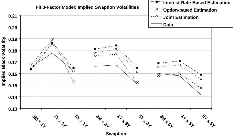
The fit on the swaptions volatilities is given in Figure 6. In case of interest-rate based
estimation and joint estimation, swaptions are overpriced by the three-factor model. The reason
for this is that the forward Libor rate correlations, as estimated using the interest rate data, are
higher than the correlations implicit in swaption prices. Since lower correlations lead to lower
swaption prices, this implies that, in case of interest-rate based estimation, swaptions are
overpriced. In case of joint estimation, there is a trade off in the fit of the covariances (or,
correlations) of forward Libor rates and the fit of swaption volatilities. In the end, the model
parameter estimates imply forward Libor rate correlations that are somewhat lower than in the
interest rate data, and swaption volatilities that are higher than the observed swaption volatilities.
Summarizing, the three-factor model is a clear improvement over the two-factor model,
fit on all four sets of moment restrictions, Libor variances, Libor covariances, cap volatilities, and
swaption volatilities, is better, and the differences between the implications of option-based
estimation and interest-rate based estimation are much smaller than in case of the two-factor
model. Only for the correlation structure of forward Libor rates and swaption prices, these two
estimation methods yield somewhat different results. The joint estimation strategy illustrates how
information in interest-rate data and option price data can be combined to accurately estimate the
three-factor model, and Table 3 confirms that, in case of joint estimation, almost all moment
restrictions are fitted accurately.
5 Summary and Conclusion
In this paper we examine multi-factor Libor Market Models. We specify a model with correlated
factors, where each factor has a volatility function that corresponds to mean-reverting behaviour
of the factor. This way, the model is related to the affine class of term structure models (Duffie
and Kan (1996)), and the stochastic mean model of Jegadeesh and Pennacchi (1996).
To estimate and test such multi-factor models, we combine the information in interest rate
data with the information in the prices of interest rate options. Previous empirical work on term
structure models has estimated and tested models on the basis of either interest rate data, or
derivative price data. In this paper, we analyze the benefits of combining these two data sets for
estimating and testing term structure models. For comparison, we also estimate the models both
only on the basis of interest rate data and only on the basis of option price data.
We use weekly US data on Libor and swap rates and prices for caps and swaptions from 1995
to 1999. The model setup explicitly allows for the presence of measurement error in both the
interest rates and derivative prices. Given the model setup, moment restrictions are derived for
both variances and covariances of changes in forward Libor rates, and for the expected prices of
caps and swaptions. Estimation is performed by applying the Generalized Method of Moments
(GMM, Hansen (1982)). We estimate both two-factor and three-factor models.
First, we analyze whether using both interest rate and option price data leads to more
accurate parameter estimates. For both the two-factor and three-factor model, we find that, when
parameter estimates are not always smaller than the standard errors that result when only interest
rate data or option price data are used for estimation.
Second, we analyze the fit of the models on the interest rate and option price data. The results
for the two-factor model show that, in case of estimation based on option prices only, the model
does not accurately fit the standard deviations of forward Libor rate changes, and, in case of
estimation on the basis of interest rate data, the model misprices caps and, especially, swaptions.
Thus, the two-factor model cannot fit the main features of the two data sets at the same time.
This result illustrates the benefit of using both interest rate data and option price data for testing
term structure models.
The three-factor model provides a better fit to both the interest rate data and the option price
data. Both the humped shape of the standard deviations of forward Libor rate changes, and the
humped shape of the cap implied volatility curve are fitted more accurately. Still, the model
slightly overprices swaptions, and the model implies correlations between forward Libor rate
changes that are a bit lower than in the data.
The results also show that allowing for measurement error in the interest rates is an important
aspect of the model setup. Neglecting this measurement error structure would lead to overpricing
of caps and too low standard deviations of forward Libor rate changes. However, although the
three-factor model gives a reasonably good fit of both the interest rate data and option price data,
the estimate for the variance of the measurement error in the forward Libor rates seems to be
unrealistically large. In this paper, we have assumed that the forward Libor measurement errors
are uncorrelated across forward Libor maturities, and have the same variance. It would be
interesting to analyze whether more realistic estimates for the size of the measurement error
References
Amin, K.I., and A. Morton (1994), ‘Implied Volatility Functions in Arbitrage-Free Term
Structure Models’, Journal of Financial Economics, 35, 141-180.
Black, F. (1976), ‘The Pricing of Commodity Contracts’, Journal of Financial Economics 3, 167-179.
Brace, A., D. Gatarek, and M. Musiela (1997), ‘The Market Model of Interest Rate Dynamics’,
Mathematical Finance 7, 27-155.
Buhler, W., M. Uhrig, U. Walter, and T. Weber (1999), ‘An Empirical Comparison of
Forward-and Spot-Rate Models for Valuing Interest-Rate Options’, Journal of Finance, 54, 269-305.
Cochrane, J.H. (2001), Asset Pricing, Princeton University Press.
Dai, Q., and K.J. Singleton (2000), ‘Specification Analysis of Affine Term Structure Models’,
Journal of Finance, forthcoming.
De Jong, F. (2000), ‘Time-series and Cross-section Information in Affine Term Structure
Models’, Journal of Economics and Business Statistics, 18 (3), 300-318.
De Jong, F., J. Driessen, and A.A.J. Pelsser (2000), ‘Libor Market Models versus Swap Market
Models for Pricing Interest Rate Derivatives: An Empirical Analysis’, Center Discussion Paper
2000-35, Tilburg University.
Driessen J., B. Melenberg, and Th.E. Nijman (1999), ‘Testing Affine Term Structure Models in
case of Transaction Costs’, Center Discussion Paper 1999-84, Tilburg University.
Duan, J., and J.G. Simonato (1999), ‘Estimating Exponential-affine Term Structure Models by
Duffee, G. (1999), ‘Estimating the Price of Default Risk’, Review of Financial Studies, 12, 197-226.
Duffie, D., and R. Kan (1996), ‘A Yield-Factor Model of Interest Rates’, Mathematical Finance,
64, 379-406.
Flesaker, B. (1993), ‘Testing the Heath-Jarrow-Morton/Ho-Lee Model of Interest Rate
Contingent Claims’, Journal of Financial and Quantitative Analysis 28, 483-495.
Gourieroux, C., and A. Monfort (1995), Statistics and Econometric Models, Cambridge University Press.
Hansen, L.P. (1982), ‘Large Sample Properties of Generalized Methods of Moments Estimators’,
Econometrica, 50, 1029-1054.
Jamshidian, F. (1997), ‘Libor and Swap Market Models and Measures’, Finance and Stochastics
1, 293-330.
Jegadeesh, N., and G.G. Pennacchi (1996), ‘The Behavior of Interest Rates Implied by the Term
Structure of Eurodollar Futures’, Journal of Money, Credit and Banking 28, 426-451.
Miltersen, K., K. Sandmann, and D. Sondermann (1997), ‘Closed Form Solutions for Term
Structure Derivatives with Lognormal Interest Rates’, Journal of Finance 52, 407-430.
Moraleda, J.M., and A.C.F. Vorst (1997), ‘Pricing American Interest Rate Claims with Humped
Volatility Models’, Journal of Banking and Finance 21, 1131-1157.
Newey, W.K., and K.D. West (1987), ‘A Simple, Positive Semi-Definite, Heteroskedasticity and
Autocorrelation Consistent Covariance Matrix’, Econometrica 55, 703-708.
Pearson, N.D., and T.S. Sun (1994), ‘Exploiting the Conditional Density in Estimating the Term
Table 1. Fit 2-Factor Models: Correlations Forward Libor Rates.
The 2-factor LMM in equations (2) and (5) is estimated using first-stage GMM on the basis of three sets of
moments as described in the text. The table reports the correlations between forward Libor rate changes of different forward maturities, as implied by the 2-factor models.
Data Interest-Rate Estimation
Maturity 1.25 2.75 4.75 9.75 1.25 2.75 4.75 9.75
0.25 0.895 0.727 0.704 0.576 0.863 0.854 0.839 0.786
1.25 - 0.847 0.832 0.688 - 0.882 0.866 0.811
2.75 - - 0.958 0.632 - - 0.858 0.803
4.75 - - - 0.821 - - - 0.789
Option Estimation Joint Estimation
Maturity 1.25 2.75 4.75 9.75 1.25 2.75 4.75 9.75
0.25 0.814 0.784 0.728 0.525 0.762 0.748 0.726 0.653
1.25 - 0.806 0.749 0.540 - 0.814 0.790 0.711
2.75 - - 0.722 0.520 - - 0.776 0.698
4.75 - - - 0.483 - - - 0.678
Table 2. Parameter Estimates 2-Factor Model.
The 2-factor LMM in equations (2) and (5) is estimated using first-stage GMM on the basis of three sets of
moments: variances and covariances of forward Libor rate changes, cap and swaption implied volatilities, and
these two sets together. The table reports parameter estimates and standard errors, which are corrected for
heteroskedasticity and 20th-lag autocorrelation using Newey-West (1987).
Interest-Rate-Based Estimation Option-Based Estimation Joint Estimation
F1 0.222 (0.019) 0.246 (0.013) 0.212 (0.010)
F2 0.131 (0.095) 0.504 (0.017) 0.484 (0.001)
61 0.064 (0.018) 0.134 (0.018) 0.066 (0.001)
62 3.234 (1.166) 8.526 (0.882) 7.617 (0.716)
D12 -0.999 -0.996 (0.052) -0.859 (0.091)
[image:26.595.75.526.587.713.2]Table 3. Average Absolute T-ratios Moment Restrictions.
For the 2-factor and 3-factor models, the t-ratios of the individual moment restrictions are calculated, correcting
for heteroskedasticity and 20th-lag autocorrelation using Newey-West (1987). The table reports for each set of
moments the average of the absolute value of these t-ratios, and the number of moment restrictions that is individually rejected at the 5% significance level.
Interest-Rate-Based
Estimation
Option-Based
Estimation
Joint Estimation
2-Factor Model
Libor Variances (9) 0.919 (0) 1.853 (2) 0.988 (1)
Libor Covariances (10) 1.670 (3) 2.593 (6) 2.201 (3)
Caps (7) 0.946 (0) 0.580 (0) 0.748 (0)
Swaptions (9) 3.973 (7) 1.318 (2) 1.801 (4)
3-Factor Model
Libor Variances (9) 0.225 (0) 0.390 (0) 0.243 (0)
Libor Covariances (10) 0.338 (0) 1.725 (3) 0.426 (0)
Caps (7) 0.443 (0) 0.317 (0) 0.439 (0)
Swaptions (9) 2.173 (4) 0.978 (1) 1.608 (3)
Table 4. Parameter Estimates 3-Factor Model.
The 3-factor LMM in equations (2) and (5) is estimated using first-stage GMM on the basis of three sets of
moment restrictions. The table reports parameter estimates and standard errors, which are corrected for
heteroskedasticity and 20th-lag autocorrelation using Newey-West (1987).
Interest-Rate-Based Estimation Option-Based Estimation Joint Estimation
F1 0.147 (0.015) 0.149 (0.045) 0.143 (0.014)
F2 0.908 (1.18) 0.508 (0.024) 0.687 (0.422)
F3 0.754 (1.17) 0.387 (0.053) 0.505 (0.448)
61 0.000 (0.008) 0.003 (0.044) 0.000 (0.016)
62 1.670 (0.566) 2.964 (1.01) 2.038 (0.656)
63 0.969 (0.450) 0.544 (0.024) 0.876 (0.344)
D12 -0.635 (0.083) -0.429 (0.633) -0.634 (0.305)
D13 -0.974 (0.090) -0.805 (0.192) -0.941 (0.103)
D23 0.529 (0.138) -0.106 (0.354) 0.486 (0.343)
[image:27.595.74.526.507.705.2]Table 5. Fit 3-Factor Models: Correlations Forward Libor Rates.
The 3-factor LMM in equations (2) and (5) is estimated using first-stage GMM on the basis of three sets of
moments as described in the text. The table reports the correlations between forward Libor rate changes of
different forward maturities, as implied by the 3-factor models.
Data Interest-Rate Estimation
Maturity 1.25 2.75 4.75 9.75 1.25 2.75 4.75 9.75
0.25 0.895 0.727 0.704 0.576 0.636 0.538 0.479 0.465
1.25 - 0.847 0.832 0.688 - 0.856 0.782 0.762
2.75 - - 0.958 0.632 - - 0.839 0.828
4.75 - - - 0.821 - - - 0.831
Option Estimation Joint Estimation
Maturity 1.25 2.75 4.75 9.75 1.25 2.75 4.75 9.75
0.25 0.665 0.428 0.191 0.059 0.596 0.501 0.444 0.428
1.25 - 0.797 0.608 0.484 - 0.837 0.760 0.738
2.75 - - 0.777 0.709 - - 0.813 0.801
Figure 1. Libor Volatilities 2-Factor Model. The 2-factor LMM (equations (2) and (5)) is estimated using first-stage GMM on the basis of three sets of moments as described in the text. The figure plots the annualized standard deviations of forward Libor rate changes, as implied by the 2-factor models.
0 1 2 3 4 5 6 7 8 9 10
0.1 0.12 0.14 0.16 0.18 0.2 0.22 0.24
Fit 2-Factor Model: Forward Libor Standard Deviations
Forward Maturity
Annualized Standard Deviation
Data
Joint
Option Interest-Rate
Figure 2. Cap Volatilities 2-Factor Model. The 2-factor LMM (equation (2) and (5)) is estimated using first-stage GMM on the basis of three sets of moments as described in the text. The figure plots the cap Black volatilities for different option maturities, as implied by the 2-factor models.
0 1 2 3 4 5 6 7 8 9 10
0.15 0.16 0.17 0.18 0.19 0.2 0.21
Fit 2-Factor Model: Cap Implied Volatilities
Cap Maturity
Implied Volatility
Data
Interest-Rate Option
[image:29.595.88.384.467.705.2]Figure 3. Swaption Volatilities 2-Factor Model. The 2-factor LMM (equations (2) and (5)) is estimated using first-stage GMM on the basis of three sets of moments as described in the text. The figure plots the swaption Black volatilities for different option maturities, as implied by the 2-factor models.
Fit 2-Factor Model: Implied Swaption Volatilities
0.13 0.14 0.15 0.16 0.17 0.18 0.19 0.20
3M x 1Y 1Y x 1Y 5Y x 1Y 3M x 3Y 1Y x 3Y 5Y x 3Y 3M x 5Y 1Y x 5Y 5Y x 5Y
Swaption
Implied Black Volatility
Interest-Rate-Based Estimation
Option-based Estimation Joint Estimation
Data
Figure 4. Libor Volatilities 3-Factor Model. The 3-factor LMM (equations (2) and (5)) is estimated using first-stage GMM on the basis of three sets of moments as described in the text. The figure plots the annualized standard deviations of forward Libor rate changes, as implied by the 3-factor models.
0 1 2 3 4 5 6 7 8 9 10
0.15 0.2 0.25
Fit 3-Factor Model: Forward Libor Standard Deviations
Forward Maturity
Annualized Standard Deviation
Data Option Interest-Rate
[image:30.595.88.386.456.692.2]Figure 5. Cap Volatilities 3-Factor Model. The 3-factor LMM (equations (2) and (5)) is estimated using first-stage GMM on the basis of three sets of moments as described in the text. The figure plots the cap Black volatilities for different option maturities, as implied by the 3-factor models.
0 1 2 3 4 5 6 7 8 9 10
0.15 0.16 0.17 0.18 0.19 0.2 0.21
Fit 3-Factor Model: Cap Implied Volatilities
Cap Maturity
Implied Volatility
Data Interest-Rate
Joint Option
Figure 6. Swaption Volatilities 3-Factor Models. The 3-factor LMM (equations (2) and (5)) is estimated using first-stage GMM on the basis of three sets of moments as described in the text. The figure plots the swaption Black volatilities for different option maturities, as implied by the 3-factor models.
Fit 3-Factor Model: Implied Swaption Volatilities
0.13 0.14 0.15 0.16 0.17 0.18 0.19 0.20 0.21
3M x 1Y 1Y x 1Y 5Y x 1Y 3M x 3Y 1Y x 3Y 5Y x 3Y 3M x 5Y 1Y x 5Y 5Y x 5Y
Swaption
Implied Black Volatility
Interest-Rate-Based Estimation
Option-based Estimation Joint Estimation
[image:31.595.77.468.480.709.2]