P-CSI v1.0, an accelerated barotropic solver for the high-resolution ocean model component in the Community Earth System Model v2.0

www.geosci-model-dev.net/9/4209/2016/ doi:10.5194/gmd-9-4209-2016

© Author(s) 2016. CC Attribution 3.0 License.

P-CSI v1.0, an accelerated barotropic solver for the high-resolution

ocean model component in the Community Earth System Model v2.0

Xiaomeng Huang1,2, Qiang Tang1, Yuheng Tseng3, Yong Hu1, Allison H. Baker3, Frank O. Bryan3, John Dennis3, Haohuan Fu1, and Guangwen Yang1

1_{Ministry of Education Key Laboratory for Earth System Modeling, and Center for Earth System Science,} Tsinghua University, Beijing, 100084, China

2_{Laboratory for Regional Oceanography and Numerical Modeling, Qingdao National Laboratory for Marine Science and} Technology, Qingdao, 266237, China

3_{The National Center for Atmospheric Research, Boulder, CO, USA}

Correspondence to:Xiaomeng Huang ([email protected]) and Yuheng Tseng ([email protected]) Received: 26 May 2016 – Published in Geosci. Model Dev. Discuss.: 1 July 2016

Revised: 3 November 2016 – Accepted: 3 November 2016 – Published: 22 November 2016

Abstract.In the Community Earth System Model (CESM), the ocean model is computationally expensive for high-resolution grids and is often the least scalable component for high-resolution production experiments. The major bot-tleneck is that the barotropic solver scales poorly at high core counts. We design a new barotropic solver to accelerate the high-resolution ocean simulation. The novel solver adopts a Chebyshev-type iterative method to reduce the global com-munication cost in conjunction with an effective block pre-conditioner to further reduce the iterations. The algorithm and its computational complexity are theoretically analyzed and compared with other existing methods. We confirm the significant reduction of the global communication time with a competitive convergence rate using a series of idealized tests. Numerical experiments using the CESM 0.1◦ global ocean model show that the proposed approach results in a factor of 1.7 speed-up over the original method with no loss of accuracy, achieving 10.5 simulated years per wall-clock day on 16 875 cores.

1 Introduction

Recent progress in high-resolution global climate models has demonstrated that models with finer resolution can bet-ter represent important climate processes to facilitate cli-mate prediction. Significant improvements can be achieved in the high-resolution global simulations of tropical

instabil-ity waves (Roberts et al., 2009), El Niño–Southern Oscilla-tion (ENSO) (Shaffrey et al., 2009), the Gulf Stream separa-tion (Chassignet and Marshall, 2008; Kuwano-Yoshida et al., 2010), the global water cycle (Demory et al., 2014), and other aspects of the mean climate and variability. Specifically, Gent et al. (2010) and Wehner et al. (2014) showed that increasing the atmosphere models’ resolution results in a better mean climate, more accurate depiction of the tropical storm forma-tion, and more realistic events of extreme daily precipitation. Bryan et al. (2010) and Graham (2014) also suggested that increasing the ocean models’ resolution to the eddy resolv-ing level helps to capture the positive correlation between sea surface temperature and surface wind stress and improves the asymmetry of the ENSO cycle in the simulation.

In the High-Resolution Model Intercomparison Project (HighResMIP) for the Coupled Model Intercomparison Project phase 6 (CMIP6), global model resolutions of 25 km or finer at mid-latitudes are proposed to implement the Tier-1 and Tier-2 experiments (Eyring et al., 20Tier-15). Because all CMIP6 climate models are required to run for hundreds of years, tremendous computing resources are needed for high-resolution production simulations. To run high-high-resolution cli-mate models practically, additional algorithm optimization is required to efficiently utilize the large-scale computing re-sources.

fully coupled climate model: the Community Earth System Model (CESM). The POP solves the three-dimensional prim-itive equations with hydrostatic and Boussinesq approxima-tions and splits the time integration into two parts: the clinic and barotropic modes (Smith et al., 2010). The baro-clinic mode describes the three-dimensional dynamic and thermodynamic processes, while the barotropic mode solves the vertically integrated momentum and continuity equations in two dimensions.

The barotropic solver is the major bottleneck in the POP within the high-resolution CESM because it dominates the total execution time on a large number of cores (Jones et al., 2005). This results from the implicit calculation of the free-surface height in the barotropic solver, which scales poorly at high core counts due to an evident global communication bottleneck inherent to the algorithm. The implicit solver al-lows a large time step to efficiently compute the fast grav-ity wave mode but requires the solution of a large elliptic system of equations. The conjugate gradient method (CG) and its variants are popular choices for implicit free-surface ocean solvers, such as MITgcm (Adcroft et al., 2016), FV-COM (Lai et al., 2010), MOM3 (Pacanowsky and Griffies, 1999), and OPA (Madec et al., 1997). However, the standard CG method has a heavy global communication overhead in the existing POP implementation (Worley et al., 2011). The latest Chronopoulos-Gear (ChronGear) (D’Azevedo et al., 1999) variant of the CG algorithm is currently used in the POP to reduce the number of global reductions. A nice overview of reducing global communication costs for the CG method can be found in the work of Ghysels and Van-roose (2014). Recent efforts to improve the performance of the CG method include a variant that overlaps the global re-duction with the matrix-vector computation via a pipelined approach (Ghysels and Vanroose, 2014). However, the im-provement is still limited when using a very large number of cores because of the remaining global reduction operations. For example, when approximately 4000 cores are used in the POP, the global reduction in the PCG (preconditioned con-jugate gradient method) and ChronGear takes approximately 74 and 68 % of the entire barotropic mode time, respectively (Hu et al., 2015). This situation will get worse with more cores.

Another way to improve the CG method is precondition-ing, which has been shown to effectively reduce the num-ber of iterations. The current ChronGear solver in the POP has benefited by using a simple diagonal preconditioner (Pini and Gambolati, 1990; Reddy and Kumar, 2013). Some paral-lelizable methods such as polynomial, approximate-inverse, multigrid, and block preconditioning have drawn much at-tention recently. High-order polynomial preconditioning can reduce iterations as effectively as incomplete LU factoriza-tion in sequential simulafactoriza-tions (Benzi, 2002). However, the computational overhead for the polynomial preconditioner typically offsets its superiority to the simple diagonal pre-conditioner (Meyer et al., 1989; Smith et al., 1992). The

approximate-inverse preconditioner, although highly paral-lelizable, requires a linear system that is several times larger than the original system to be solved (Smith et al., 1992; Bergamaschi et al., 2007), making it less attractive for the POP.

Multigrid methods are well-known scalable and efficient approaches for solving elliptic systems of equations. Recent works indicated that geometric multigrid is promising in at-mosphere and ocean modeling (Müller and Scheichl, 2014; Matsumura and Hasumi, 2008; Kanarska et al., 2007). How-ever, geometric multigrid in global ocean models does not always scale ideally because of the presence of complex to-pography and non-uniform or anisotropic grids (Fulton et al., 1986; Stüben, 2001; Tseng and Ferziger, 2003; Matsumura and Hasumi, 2008). The current POP, which employs gen-eral orthogonal grids to avoid the pole singularity, is a typical example. This leads to an elliptic system with variable co-efficients defined on an irregular domain with non-uniform grids. Algebraic multigrid (AMG) is an alternative to geo-metric multigrid to handle complex topography. However, the AMG setup in the parallel environment is more expensive than the iterative solver in climate modeling, which makes it unfavorable as a preconditioner (Müller and Scheichl, 2014). Block preconditioning has been shown to be an effec-tive parallel preconditioner (Concus et al., 1985; White and Borja, 2011) and is appealing for the POP because it uses the block structure of the coefficient matrix that arises from the discretization of the elliptic equations. This advantage can further improve solver parallel performance. Some other algorithmic approaches also attempt to improve the parallel performance of ocean models. For example, a load-balancing algorithm based on the space-filling curve was proposed that not only eliminates land blocks but also reduces the commu-nication overhead due to the reduced number of processes (Dennis, 2007; Dennis and Tufo, 2008). Beare and Stevens (1997) also proposed increasing the number of extra halos and communication overlaps in the parallel ocean general circulation. Although these approaches improve the perfor-mance of ocean models, the global communication bottle-neck still exists.

To improve the scalability of the POP at high core counts, we abandon the CG-type approach and design a new barotropic solver that does not include global communica-tion in iteracommunica-tion steps. The new barotropic solver, named P-CSI, uses a classical Stiefel iteration (CSI) method (proposed originally in Hu et al., 2015) with an efficient block precon-ditioner based on the error vector propagation (EVP) method (Roache, 1995). The P-CSI solver is now the default ocean barotropic solver for the upcoming CESM 2.0 release.

POP. In particular, the characteristics of P-CSI are theoret-ically analyzed via the associated eigenvalues and their im-pacts on the spectrum, condition number, and convergence rate. In addition, we provide a more comprehensive review of barotropic modes and the existing solvers used in the de-fault POP (only a simplified discussion is provided in the SC paper). Finally, because the target audience is now ocean climate modelers, all figures have been adjusted to address the major advantages of the proposed method and the overall performance of the high-resolution POP.

The remainder of this paper is organized as follows. tion 2 reviews the existing barotropic solver in the POP. Sec-tion 3 details the design of the P-CSI solver, followed by an analysis of the computational complexity and convergence rate of P-CSI in Sect. 4. Section 5 further compares the high-resolution performance of the existing solvers and the P-CSI solvers. Finally, conclusions are given in Sect. 6.

2 Barotropic solver background

We briefly describe the governing equations to formally de-rive the new P-CSI solver in the POP. The primitive momen-tum and continuity equations are expressed as

∂

∂tu+L(u)+f×u= −

1

ρ0

∇p+FH(u)+FV(u), (1)

L(1)=0, (2)

whereL(α)= ∂

∂x(uα)+ ∂ ∂y(vα)+

∂

∂z(wα), which is equiv-alent to the divergence operator when α=1; x, y, and z

are the horizontal and vertical coordinates; u= [u, v]T is the horizontal velocity; w is the vertical velocity;f is the Coriolis parameter;pandρ0represent the pressure and the constant reference water density, respectively; FH and FV are the horizontal and vertical dissipative terms, respectively (Smith et al., 2010). In particular, we emphasize the two-dimensional barotropic mode in the time-splitting scheme, where the P-CSI is implemented.

2.1 Barotropic mode

POP uses the splitting technique to solve the barotropic and baroclinic systems (Smith et al., 2010). The governing equa-tions for the barotropic mode can be obtained by vertically integrating Eqs. (1) and (2) from the ocean bottom topogra-phy to the sea surface:

∂U

∂t = −g∇η+F, (3)

∂η

∂t = −∇ ·HU+qw, (4)

whereU= 1

H+η

Rη

−Hdzu(z)≈ 1 H

R0

−Hdzu(z)is the vertically integrated barotropic velocity,gis the gravity acceleration,η

is the sea surface height (defined asps/ρ0g, whereps is the

surface pressure associated with undulations of the free sur-face),His the depth of the ocean bottom,qwis the freshwa-ter flux per unit area, andFis the vertical integral of all other terms except the time-tendency and surface pressure gradi-ent in the momgradi-entum Eq. (1). When we directly integrate the continuity equation from the bottom to the surface, we will get a formRη

−Hdz(∇ ·u+ ∂w

∂z)= ∂η

∂t + ∇ ·(H+η)U−qw= 0 under the surface boundary condition w(η)=dη

dt −qw= ∂η

∂t +u(η)· ∇η−qw. The term includingηinside the diver-gence leads to a nonlinear elliptic system, which cannot be solved by many mature numerical methods such as the con-jugate gradient methods. To avoid this, POP linearizes the continuity equation by dropping the divergence term in the boundary condition, which becomesw(η)=∂η

∂t −qw. Equa-tion (4) is the resulting barotropic continuity equaEqua-tion, and more details can be found in Smith et al. (2010).

All terms in Eq. (1) use the explicit scheme, with the ex-ception of the implicit treatment of barotropic mode and the semi-implicit treatment of the Coriolis and vertical mixing terms. Because of the restriction of barotropic CFL num-ber (defined as CFL=c·τ

1x, where c=

√

gH is the fastest speed in barotropic mode, andτ and1x are the step sizes in time and space, respectively), the implicit treatment of the barotropic mode is necessary to simulate the fast grav-ity waves with a speed ofc=200 m s−1so that we can use the same time step as the baroclinic mode, which has a ve-locity scale of less than 2 m s−1(Hu et al., 2015). Solving the barotropic mode with an implicit method allows for a much larger time step than with an explicit method. For example, with the 0.1◦POP model, an implicit method can use a time step of 172.8 s; otherwise, it would be only 1.73 s.

Equations (3) and (4) are then discretized in time using an implicit scheme as follows:

Un+1−Un

τ = −g∇η

n+1_{+F, (5)}

ηn+1−ηn

τ = −∇ ·HU

n+1_+q

w, (6)

whereτ is the time step associated with the time advance scheme. By replacing the barotropic velocity in Eq. (6) with the barotropic velocity at the next time step in Eq. (5), an elliptic system of sea surface heightηis obtained:

[−∇ ·H∇ + 1 gτ2]η

n+1_{= −∇ ·H[}Un

gτ + F

g]+ ηn gτ2+

qw

gτ. (7)

For simplicity, we can rewrite the elliptic Eq. (7) as

[−∇ ·H∇ + 1 gτ2]η

n+1_{=ψ (η}n_{, τ ), (8)}

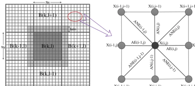
whereψrepresents a function of the current state ofη. Spatially, the POP utilizes the Arakawa B-grid on the hori-zontal grid (Smith et al., 2010) with the following nine-point stencils to discretize Eq. (8) as follows (see Fig. 1):

∇ ·H∇η= 1

1yδx[1yH δxη

y_]y₊ 1

1xδy[1xH δyη

Nx

Ny

halo

X(i+1,j)

AN E(i-1

,j-1)

A_N E(i_-1

,j)

A_N E(i_,j-1

)

AE(i-1,j)

AE(i,j)

A

N

(i

,j

)

A

N

(i

,j

-1

)

AN E(i,j

)

X(i-1,j+1) X(i,j+1) X(i+1,j+1)

X(i-1,j-1) X(i,j-1) X(i+1,j-1) X(i-1,j)

B(k,l+1)

B(k+1,l)

B(k,l-1) B(k,l)

B(k-1,l) X(i,j)

Figure 1.Grid domain decomposition of the ocean model component in CESM.

where δξ (ξ∈ {x, y}) are finite differences and 1ξ (ξ ∈

{x, y}) are the associated grid lengths. The finite difference

δξ(ψ )and averageψ ξ

notations are defined, respectively, as follows:

δξψ= [ψ (ξ+1ξ/2)−ψ (ξ−1ξ/2)]/1ξ, (10)

ψξ = [ψ (ξ+1ξ/2)+ψ (ξ−1ξ/2)]/2. (11)

Because the POP uses general orthogonal grids, the coef-ficient matrix varies in space. To demonstrate the properties of the sparse matrix used in the POP, we can simplify Eq. (9) using a special case with uniform grids as follows:

[∇ ·H∇η]_i,j = (12)

− 1 Si,j

h

BOH ηi,j+BNWHi−1,jηi−1,j+1

+1

2B N_(H

i,j+Hi−1,j)ηi,j+1

+BNEHi,jηi+1,j+1+ 1 2B

W_(H i−1,j

+Hi−1,j−1)ηi−1,j+ 1 2B

E_(H

i,j+Hi,j−1)ηi+1,j

+BSWHi−1,j−1ηi−1,j−1+ 1 2B

S_(H i,j−1

+Hi−1,j−1)ηi,j−1+BSEHi,j−1ηi+1,j−1

i

,

where Si,j =1x1y and H=1₄(Hi,j+Hi−1,j+Hi,j−1+

Hi−1,j−1); theH inside this equation is the ocean bottom depth in the columns of U-points (Smith et al., 2010). The

Bs are determined using1x and1y:

α=1y

1x, β=1/α, (13)

BNW=BNE=BSW=BSE= −(α+β)/4, BW=BE=(β−α)/2,

BN=BS=(α−β)/2, BO=α+β.

To make the discretization of Eq. (8) more succinct, notations are introduced as follows:

AO_i,j =BOH , (14)

AN_i,j =1

2B N_(H

i,j+Hi−1,j),

AW_i,j =1

2B W_(H

i−1,j+Hi−1,j−1),

AE_i,j =1

2B E_(H

i,j+Hi,j−1),

AS_i,j =1

2B S_(H

i,j−1+Hi−1,j−1),

ANW_i,j =BNWHi−1,j, ANEi,j =B NE_H

i,j,

ASW_i,j =BSWHi−1,j−1, ASEi,j=BSEHi,j−1.

TheseAχ_i,j(χ∈Q= {O, NW, NE, SW, SE, W, E, N, S}) are coefficients between a grid point(i, j )and its neighbors us-ing the nine-point stencil discretization (Eq. 9).

The full discretization of Eq. (8) for any given grid point

(i, j )can then be written as

(AO_i,j+φ)ηi,j+ANWi,j ηi−1,j+1+ANi,jηi,j+1 (15)

+ANE_i,jηi+1,j+1+AWi,jηi−1,j

+AE_i,jηi+1,j+A_i,jSWηi−1,j−1+AS_i,jηi,j−1

+ASE_i,jηi+1,j−1=Si,jψi,j, whereφ=Si,j

0 100 200 300 400

nz = 3870

0

50

100

150

200

250

300

350

400

450

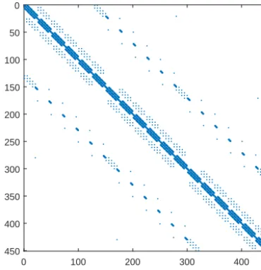
Figure 2.Sparsity pattern of the coefficient matrix in the case with 30×15 grids using nine-point stencils.

Therefore, the elliptic Eq. (7) leads to a linear system of

η, i.e.,Ax=b, whereAis a block tridiagonal matrix com-posed of coefficients Aχ_i,j(χ∈Q). The simplified equation set of Eqs. (13), (14) and (15) shows that Ais mainly de-termined by the horizontal grid sizes, ocean depth and time step. These impacts will be further discussed in Sect. 4.1. Note that Eq. (15) also indicates that the sparsity pattern of Acomes directly from the nine nonzero elements in each row (Fig. 2).

POP divides the horizontal domain into small blocks evenly and distributes them to processes. We assume that there are N andM grids along longitude and latitude, re-spectively, and the global domain is divided inton·msmall blocks with a size of N_n ·M

m. These blocks are distributed to processors using a simple Cartesian strategy or space-filling curve method (Smith et al., 2010).

2.2 Barotropic solvers

The barotropic solver in the original POP uses the PCG method with a diagonal preconditioner M=3(A)because of its efficiency in small-scale parallelism (Dukowicz and Smith, 1994) (see Appendix B1 for the details). To mitigate the global communication bottleneck, ChronGear, a variant of the CG method proposed by D’Azevedo et al. (1999), was later introduced as the default solver in the POP. It combines the two separated global communications of a single scalar into a single global communication (see Appendix B2). By this strategic rearrangement, the ChronGear method achieves a one-third latency reduction in the POP. However, the scal-ing bottleneck still exists in the high-resolution POP usscal-ing this solver, particularly with a large number of cores (Fig. 3). To accurately profile the parallel cost of the barotropic solvers, we clearly separate the timing for computation, halo

Figure 3.Number of unknowns per processor and percentage of ex-ecution time in 0.1◦POP using the default diagonal-preconditioned ChronGear solver on Yellowstone.

exchange, and global reduction. Operations such as scalar computations and vector scalings are categorized as pure computations, which are relatively cheap due to the indepen-dent operations on each process. The extra halo exchange is required for each process to update the boundary values from its neighbors (Fig. 1) after the matrix-vector multipli-cation. This halo exchange usually costs more than the com-putation when a large number of cores is used (due to a de-creasing problem size per core). The global reduction, which is needed by the inner products of vectors, is even more costly (Hu et al., 2013). Worley et al. (2011) and Dennis et al. (2012) specifically indicated that the global reduction in the POP’s barotropic solver is the main scaling bottleneck for the high-resolution ocean simulation.

Figure 3 confirms that the percentage of execution time for the barotropic mode in 0.1◦POP indeed increases with an in-creasing number of processor cores on Yellowstone. When 470 cores are used, the execution time of the barotropic solver is approximately 5 % of the total execution time (ex-cludes initialization and I/O). However, when several thou-sand cores are used, the percentage of time spent in the baro-clinic mode decreases, associated with the increasing per-centage of time in the barotropic solver. With more than 16 000 cores, the percentage of the total execution time due to the barotropic solver is nearly 50 %.

3 Design of the P-CSI solver

a new solver targeted for reducing global communication so that the speed-up can be as close to unity as possible when a significant number of cores are used.

3.1 Classical Stiefel iteration method

The CSI is a special type of Chebyshev iterative method (Stiefel, 1958). Saad et al. (1985) proposed a generalization of CSI on linearly connected processors and claimed that this approach outperforms the CG method when the eigen-values are known. This method was revisited by Gutknecht and Röllin (2002) and shown to be ideal for massively par-allel computers. In the procedure of preconditioned CSI (P-CSI; details are provided in Appendix B3), the iteration pa-rameters, which control the searching directions in the iter-ation step, are derived from a stretched Chebyshev function of two extreme eigenvalues (Stiefel, 1958). We demonstrate in Sect. 4.2 that the stretched Chebyshev function in P-CSI provides a series of preset parameters for iteration directions. As a result, P-CSI requires no inner product operation, thus potentially avoiding the bottleneck of global reduction. This makes the P-CSI more scalable than ChronGear on massively parallel architectures. However, it requires a priori knowl-edge about the spectrum of coefficient matrixA(Gutknecht and Röllin, 2002). It is well known that obtaining the eigen-values of a linear system of equations is equivalent to solv-ing it. Fortunately, the coefficient matrixAand its precondi-tioned form in the POP are both positive-definite real sym-metric matrices. Approximate estimation of the largest and smallest eigenvalues,µandν, respectively, of the precondi-tioned coefficient matrix is sufficient to ensure the conver-gence of P-CSI.

To efficiently estimate the extreme eigenvalues of the pre-conditioned matrixM−1A(whereMis the preconditioner), we adopt the Lanczos method (Paige, 1980) (see the algo-rithm in Appendix C). Initial tests indicate that only a small number of Lanczos steps are necessary to reasonably esti-mate the extreme eigenvalues ofM−1Athat result in near-optimal P-CSI convergence (Hu et al., 2015). Therefore, the computational overhead of the eigenvalue estimation is very small in our algorithm.

3.2 A block EVP preconditioner

Block preconditioning is quite promising in the POP because parallel domain decomposition is ideal for the block struc-ture. A block preconditioning based on the EVP method is proposed and detailed in Hu et al. (2015); it improves the parallel performance of the barotropic solver in the POP. To the best of our knowledge, the EVP and its variants are among the least costly algorithms for solving elliptic equa-tions in serial computation (Roache, 1995) and have also been used in several different ocean models (Dietrich et al., 1987; Sheng et al., 1998; Young et al., 2012). The paral-lel EVP solver was also implemented by Tseng and Chien

(2011). The standard EVP is actually a direct solver, which requires two solution steps: preprocessing and solving. In the preprocessing stage, the influence coefficient matrix and its inverse are computed, involving a computational complex-ity ofCpre=(2n−5)·9n2+(2n−5)3=O(26n3), which is intensive but computed only once at the beginning. The solv-ing stage is computed at every time step and requires only

Cevp=2·9n2+(2n−5)2=O(22n2)(Hu et al., 2015), which is a much lower computational cost than those of other direct solvers, such as LU.

The EVP method is efficient for solving elliptic equa-tions. Although EVP preconditioning may increase the re-quired computation for each iteration, the barotropic solver can greatly benefit from the resulting reduction in the num-ber of iterations, particularly at very large numnum-bers of cores when communication costs dominate (Hu et al., 2015). For large-scale parallel computing, a larger number of proces-sors typically results in smaller domains, which in fact favors the application of the EVP method (Dietrich, 1975; Roache, 1995). If the domain size is too large without using domain decomposition, the computation will be very slow (see the complexity analysis in Sect. 4.3 whenp=1). Using paral-lel domain decomposition can actually help and speed up the EVP solver.

4 Algorithm analysis and comparison

The extreme eigenvalues of the coefficient matrix are critical to determine the convergence of the iterative solvers (such as P-CSI, PCG and ChronGear). Here, the characteristics of P-CSI are investigated in terms of the associated eigenvalues and their connection with the convergence rate. The compu-tational complexity is also addressed.

4.1 Spectrum and condition number

Because the coefficient matrix A in the POP is symmet-ric and positive-definite (Smith et al., 2010), its eigenval-ues are positive real numbers (Stewart, 1976). We assume that the spectrum (Golub and Van Loan, 2012) ofAisS= {λ1, λ2, . . ., λN}, where λmin=λ1≤λi≤λN =λmax (1<

i <N; N is the size of A) are the eigenvalues of A. The condition number, defined asκ=λmax/λmin, is determined based on the spectral radius. Using the Gershgorin circle the-orem (Bell, 1965), we know that for anyλ∈S, there exists a pair of(i, j )satisfying

|λ−(AO_i,j+φ)| ≤ X

χ∈Q−{O}

|Aχ_i,j|, (16)

whereφ= S

10-2 10-1 100 CFL number 100

101 102 103

Condition number

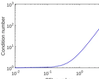
Figure 4. Relationship between the CFL number and the condi-tion number of the coefficient matrix, where the CFL number varies from 10−2to 5.

λmax≤(4max(α, 1

α)+8)max(H ), (17)

λmin≥(2min(α− 1

α,

1

α−α)+8)max(H ),

where8= φ

max(H ) and where max(H )is the maximal depth of the ocean bottom; for more details, refer to Appendix A,

To quantitatively evaluate the impacts of the condition number, we set up a series of idealized test cases to solve Eq. (8) in which the coefficient matrices are derived from Eqs. (13), (14) and (15) on an idealized cylinder with an earth-sized perimeter, which is 2π R(radiusR is 6372 km), and a height ofπ R. A uniform grid with a size ofN×Mis used, where the grid size along the perimeter and height are

1x=2π R/Nand1y=π R/M, respectively. The depthH

is set as a constant 4 km to simplify the analysis.

The inequalities Eq. (17) suggest that the lower bound of the eigenvalues is mostly determined by 8. If we assume that the grid aspect ratio is unity, we can rewrite8= S

gτ2_H as 8= 1

(CFL)2 in terms of the barotropic CFL number (as defined in Sect. 2.1). This indicates that, for a given ocean configuration and grid size, the lower bound of the eigenval-ues will decrease with increasing CFL number, resulting in a larger condition number. Figure 4 shows the relationship between condition number and the CFL number. In this ide-alized test case, 8becomes very large and dominates both

λmax andλmin when the CFL number is sufficiently small (smaller than 10−1s). As a result, the condition number proaches 1. When the CFL number is large enough (i.e., ap-proaches 5), the condition number is highly determined by the grid aspect ratioαbecause of the reduced impact of8.

When the aspect ratio of the horizontal grid cell ap-proaches unity, the upper (lower) bound of the largest (small-est) eigenvalue decreases (increases), leading to a reduced spectral radius ([λmin, λmax]). This implies that the condi-tion number is also reduced simultaneously. Figure 5 shows

10-2 10-1 100 101 102

Aspect ratio " x /" y 0

30 60 90 120

Condition number CFL = 0.5

CFL = 1 CFL = 3.46 CFL = 5

Figure 5.Relationship between the aspect ratio and the condition number of the coefficient matrix under the condition of different typical CFL numbers.

the condition number vs. the aspect ratio, which is consis-tent with the theoretical bounds of the extreme eigenvalues in Eq. (17). As expected, the smallest condition number is found in Fig. 5 when the grid aspect ratio approaches unity regardless of the CFL number. When the aspect ratio equals unity (i.e., α=1y

1x=1), we obtain λmax≤(4+8)H and

λmin≥8H.

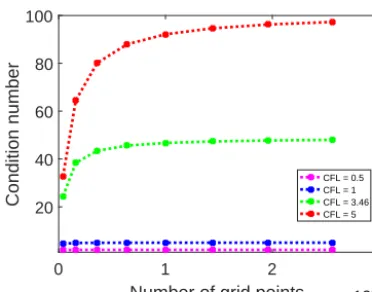
Our analysis suggests that the spectral radius is confined in(8H, (4+8)H )if the aspect ratio is unity regardless of grid sizes. However, the condition number may vary greatly because of the dependency on the grid sizeN and the aspect ratio. When the grid sizeN increases, the largest eigenvalue remains close to 4H, whereas the smallest eigenvalue be-comes closer to8H. Therefore, the condition number is sig-nificantly affected when the aspect ratio is far from unity. To focus on the impact of the number of grid points, we choose a constant aspect ratioα=1. Figure 6 shows that the condition number increases monotonically with increasing grid size for the four given different CFL conditions. It also shows that the CFL number has a large impact on the condition number.

In the 0.1◦ POP simulation, the CFL number is ap-proximatelyc·1t /1x≈3.46 (wherec=200 m s−1,1t=

172.8 s, and 1x=10 000 m are the typical gravity wave speed, time step, and spatial resolution, respectively) and the condition number is approximately 250. For comparison, the condition number in the 1◦POP simulation is higher, which is approximately 1200.

4.2 Convergence rate

0 1 2 3

Number of grid points #104

20 40 60 80 100 Condition number

CFL = 0.5 CFL = 1 CFL = 3.46 CFL = 5

Figure 6.When the aspect ratio is constantα=1, the relationship between the number of grid points and the condition number of the coefficient matrix under the condition of different typical CFL num-bers.

as follows (Liesen and Tichý, 2004):

||xk−x∗||A0

||x0−x∗||A0

≤ min

p∈Pk,p(0)=1

max

λ∈S|p(λ)|, (18)

wherexk is the solution vector after thekth iteration,x∗is the solution of the linear equation (i.e., x∗_=A−1_b),λ rep-resents an eigenvalue of A0_{, and P}

k is the vector space of polynomials with real coefficients and a degree less than or equal tok. Applying the Chebyshev polynomials of the first type to estimate this min–max approximation, we obtain

||xk−x∗||A0≤2( √

κ−1

√ κ+1)

k_||x

0−x∗||A0, (19)

whereκ=κ2(A0)= λ0

max

λ0_min is the condition number of matrix A0 with respect to thel2norm. Equation (19) indicates that the theoretical bound of the convergence rate of PCG de-creases with increasing condition number. PCG converges faster for a well-conditioned matrix (e.g., a matrix with a small condition number) than an ill-conditioned matrix.

We now show that the P-CSI has the same order of conver-gence rate as PCG and ChronGear with the additional advan-tage of fewer global reductions in parallel computing. With the estimated smallest and largest extreme eigenvalues of co-efficient matrixνandµ, the residual for the P-CSI algorithm satisfies

rk=Pk(A0)r0, (20)

wherePk(ζ )=τk(β−αζ )_τk(β) for ζ ∈ [ν, µ](Stiefel, 1958), α= 2

µ−ν and β= µ+ν

µ−ν. τk(ξ ) is a Chebyshev polynomial ex-pressed as

τk(ξ )= 1 2

"

ξ+

q

ξ2₋₁

k

+

ξ+

q

ξ2₋₁

−k#

. (21)

Whenξ∈ [−1,1], the Chebyshev polynomial has an equiv-alent form

τk(ξ )=cos(kcos−1ξ ), (22)

which clearly shows that|τk(ξ )| ≤1 when|ξ| ≤1.Pk(ζ )is the polynomial satisfying

Pk= min p∈Pk,p(0)=1

max ζ∈[ν,µ]

|p(ζ )|. (23)

Assume thatA0=QT3Q, where 3is a diagonal matrix having the eigenvalues ofA0on the diagonal andQis a real orthogonal matrix with columns that are eigenvectors ofA0. We then have

Pk(A0)=QTPk(3)Q (24)

=QT

    

Pk(λ1)

Pk(λ2)

. ._.

Pk(λN)

     Q.

Assuming that ν and µ satisfy 0< ν≤λi≤µ (i= 1,2, . . .,N), Eq. (22) indicates that |β−αλi| ≤1 and

|Pk(λi)| =τk(β−αλ_τ i)

k(β) ≤τ

−1

k (β). Equations (20) and (24) in-dicate that

||rk||2

||r0||2

≤τ_k−1(β)= 2(β+

p

β2₋₁₎k

1+(β+pβ2₋₁₎2k (25)

≤2( √

κ0₋₁

√ κ0₊₁)

k_,

whereκ0=µ

ν. Equation (25) shows that P-CSI has the same theoretical upper bound of the convergence rate as PCG and ChronGear when the estimation of eigenvalues is appropriate (e.g.,κ0=κ).

The foregoing analysis applies to cases in which a non-trivial preconditioning is used. Assume that the precondi-tioned coefficient matrixA0=M−1A. Note that the precon-ditioned matrix in the PCG, ChronGear and P-CSI algo-rithms is actuallyM−1/2_A(M−1/2₎T_{, which is symmetric and} has the same set of eigenvalues asM−1_{A(Shewchuk, 1994).} Thus, the condition number of the preconditioned matrix is

κ=κ2(M−1/2A(M−1/2)T), which is usually smaller than the condition number ofA. The closerMis toA, the smaller the condition number ofM−1Ais. WhenMis the same as A, thenκ2(M−1A)=1.

4.3 Computational complexity

To analyze the computational complexity of P-CSI and com-pare it with ChronGear, we definep as the number of pro-cesses andN as the number of grid points (using the same notation as in Hu et al., 2015). Both the ChronGear and P-CSI solver time can then be divided into three major com-ponents: computation Tc, halo exchanging Tb, and global communication Tg. The complexity of computation varies among different solvers and preconditioners. The halo ex-change complexity is Tb=O(4$+8

q

N

pϑ ), where $ is the ratio of point-to-point communication latency per mes-sage to the time of one floating-point operation andϑis the ratio of the transfer time per byte (inverse of bandwidth) to the time of one floating-point operation. All halo exchange times show a similarly decreasing trend with increasing num-ber of processes, but have a lower bound of 4$. The global communication exists only in the ChronGear solver and con-tains one global reduction per iteration, resulting from the MPI_Allreduce and a masking operation that excludes land points. The cost of the masking operation decreases with in-creasing processes p, whereas the cost of MPI_Allreduce monotonically increases; thus, the global reduction complex-ity satisfiesTg=O(2N_p +logp$ ).

The execution time of one diagonal preconditioned ChronGear solver step can then be expressed as

Tcg=Kcg(Tc+Tb+Tg) (26)

=O Kcg 18

N

p +8

s

N

pϑ+(4+logp)$

!!

,

whereKcgis the number of iterations, which does not change with the number of processes (Hu et al., 2015). The complex-ity of P-CSI with a diagonal preconditioner is

Tpcsi=O Kpcsi 12

N

p +8

s

N

pϑ+4$

!!

, (27)

whereKpcsiis the number of iterations.

Equation (26) indicates that the computation and halo ex-change time decrease with increasing numbers of processes. However, the time required for the global reduction increases with increasing numbers of processes. Therefore, we can ex-pect the execution time of the ChronGear solver to increase when the number of processors exceeds a certain threshold. Our analysis shows that P-CSI has a lower computational complexity than that of ChronGear due to the lack of a logp

term associated with global communications.

We further consider the computational complexity of pre-conditioning. The EVP preconditioning hasO(22N_p). Thus, with the EVP preconditioning, the computational complexity of ChronGear and P-CSI becomes O(39N_p)andO(33N_p), respectively. As a result, the total complexities of ChronGear

and P-CSI with EVP preconditioning are

Tcg−evp=O

Kcg−evp

39N

p +8

s

N

pϑ (28)

+(4+logp)$

,

Tpcsi−evp=O Kpcsi−evp 33

N

p +8

s

N

pϑ+4$

!!

. (29)

Although the computation time in each iteration doubles with the EVP preconditioning, the total time may still decrease if the number of iterations is reduced. Indeed, with EVP pre-conditioning, the number of iterationsKpcsi−evpdecreases by almost one-half (see Fig. 8). As a result, the total number of communications, which is the most time-consuming part for a large number of cores, decreases by approximately one-half.

5 Numerical experiments

To evaluate the new P-CSI solver, we first demonstrate its characteristics and compare it with PCG (and thus ChronGear) using an idealized test case. The actual perfor-mance of P-CSI in the CESM POP is then evaluated and compared with that of the existing solvers using the 0.1◦ high-resolution simulation.

5.1 Condition number and convergence rate

To confirm the theoretical analysis of the convergence in Sect. 4.2, we created a series of matrices with the ideal-ized setting illustrated in Sect. 4.1. Instead of a cylindri-cal grid, we choose a sphericylindri-cal grid with two polar conti-nents (ocean latitude varies from 80◦S to 80◦N). A uni-form latitude–longitude grid is used in which the grid size along the longitude varies with latitude coordinateθ, that is,

1x=(2π R/N )cosθ. The barotropic CFL number is set as CFL=3.46 (a typical value for a 0.1◦POP simulation, as discussed in Sect. 2.1). These cases differ with respect to the number of grid points; thus, the condition numbers vary. We compare the results using PCG and P-CSI solvers with no preconditioning, diagonal preconditioning or EVP precondi-tioning. Here, the block size in EVP preconditioning is set as 5×5 and the convergence tolerance is tol=10−6. We note that the theoretical convergence rates of ChronGear and PCG are identical; thus, the results here also apply to ChronGear.

0 1000 2000 3000 4000 Number of grid points

20 40 60 80

Number of Iterations

CG PCG(diagonal) PCG(EVP) CSI P-CSI (diagonal) P-CSI (EVP)

Figure 7.Relationship between grid sizes and number of iterations of different solvers in test cases with the idealized configuration.

better conditioned than the matrix without preconditioning or with diagonal preconditioning. As shown in the previous section, the P-CSI has the same theoretical lower bound of the convergence rate as PCG and ChronGear when the esti-mation of extreme eigenvalues is appropriate (k0=k). How-ever, P-CSI commonly has a slower convergence rate than that of PCG if the same preconditioning is applied (Fig. 7). Because P-CSI requires that 0< ν < λi< µ(i=1, . . ., N ), which means thatk0=µ/ν≥λmax/λmin=k, Eqs. (19) and (25) suggest that the P-CSI will converge more slowly than the PCG unless the estimation of extreme eigenvalues is op-timal. Furthermore, the theoretical bound is often too conser-vative for PCG as the problem size increases in application, which is not completely linear (known as superlinear conver-gence of the PCG method; Beckermann and Kuijlaars, 2001). Note that the diagonal preconditioner only slightly improves the convergence in our idealized cases because of the uni-form grid and the constant ocean depth configuration.

If the condition numbers are very large, any advanced pre-conditioner that can quickly reduce the iteration count will be very useful for improving performance. In fact, the EVP solver is a direct fast solver; thus, it is very suitable as the preconditioner within each block. It is also simple enough to effectively reduce the condition number of the coefficient matrix by approximately 5 times in both 1 and 0.1◦ cases, leading to a 2/3 reduction in the number of iterations. Even so, further studies regarding the preconditioner in practical climate models will be very useful and will be our future work.

5.2 A practical application using the high-resolution CESM POP

5.2.1 Experiment platform and configuration

We evaluate the performance of P-CSI in CESM1.2.0 on the Yellowstone supercomputer, located at NCAR-Wyoming Su-percomputing Center (NWSC) (Loft et al., 2015). Yellow-stone uses Intel Xeon E5-2670 (Sandy Bridge: 16 cores at

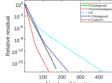
100 200 300 400 500

Number of iterations 10-15

10-12 10-9 10-6 10-3 100

Relative residual

PCG(diagonal) ChronGear(diagonal) CSI

P-CSI(diagonal) P-CSI(EVP)

Figure 8.The convergence rate of different barotropic solvers with diagonal preconditioners and the convergence rate of CSI solvers with different preconditioners in the 0.1◦POP on Yellowstone.

2.6 GHz, hyperthreading enabled, 20 MB shared L3 cache) and provides a total of 72 576 cores connected by a 13.6 GBps InfiniBand network. More than 50 % of Yellow-stone’s cycles are consumed by CESM. Therefore, the abil-ity to accelerate the parallel performance on Yellowstone is critical to support the CESM production simulations.

To emphasize the advantage of P-CSI, we use the finest 0.1◦ grid and a POP with 60 vertical levels with the “G_NORMAL_YEAR” configuration, which uses active ocean and sea ice components (i.e., the atmosphere and land components are replaced by pre-determined forcing data sets). The I/O optimization is another important issue for the high-resolution POP (Huang et al., 2014) but is not addressed here.

The choice of ocean block size and layout has a large im-pact on performance for the high-resolution POP because it directly affects the distribution of the workload among pro-cessors. To remove the influence of different block distribu-tions on our results, we carefully specify block decomposi-tions for each core with the same ratio. The time step is set to the default of 172.8 s. For a fair comparison among solvers, the convergence is checked every 10 iterations for all tests. The impacts of CSI and the EVP preconditioner are evaluated separately using several different numerical experiments.

5.2.2 Overall performance of P-CSI

1000 2000 3000 4000 5000 6000 7000 0

2 4 6 8 10 12 14 16 18 20

Global reduction

Processor cores

Execution time(s)

PCG ChronGear P−CSI P−CSI + diagonal P−CSI + EVP

1000 2000 3000 4000 5000 6000 7000 0

2 4 6 8 10 12 14 16 18 20

Halo exchanging

Processor cores PCG ChronGear P−CSI P−CSI + diagonal P−CSI + EVP

1000 2000 3000 4000 5000 6000 7000 0

2 4 6 8 10 12 14 16 18 20

Computation

Processor cores PCG ChronGear P−CSI P−CSI + diagonal P−CSI + EVP

Figure 9.The execution time for different phases using different barotropic solvers and the execution time for different phases with different preconditioners in the P-CSI solver in 0.1◦POP.

thus supporting the same upper bound for the convergence rate, as discussed in Sect. 4.2.

Figure 9 further evaluates the solver time for the differ-ent phases. P-CSI outperforms ChronGear primarily because it only requires a few global reductions in the convergence check. No significant differences can be found for the halo exchange and the computation phases when using large core counts, except for the evident reduction in execution time for the halo exchange with the EVP preconditioner. The reduc-tion in global communicareduc-tions will also significantly reduce the sensitivity of the ocean model component to operating system noise (Ferreira et al., 2008) by increasing the time interval between global synchronizations.

According to Fig. 8, the P-CSI solver can reach the same relative residual using many fewer iterations with the EVP preconditioner. As a result, it reduces not only the execu-tion time of global reducexecu-tion, but also the execuexecu-tion time of halo exchange owing to the reduced iterations which are il-lustrated in Fig. 9. All of these results are consistent with the theoretical analysis in Sect. 4.3. Note that the extra computa-tion operacomputa-tions required by the EVP precondicomputa-tioner have only a small impact on the overall performance of the barotropic solver.

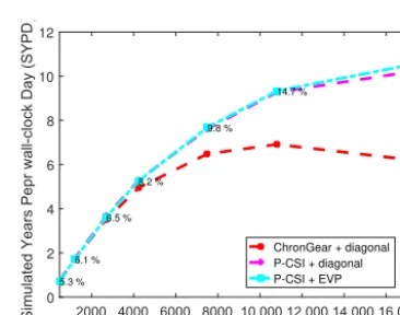
The overall performance of P-CSI in a realistic 0.1◦POP simulation is illustrated in Fig. 10. Using the EVP pre-conditioner, P-CSI can accelerate the barotropic calculation from 6.2 SYPD (simulated years per wall-clock day) to 10.5 SYPD on 16 875 cores. Dennis et al. (2012) indicated that 5 simulated years per wall-clock day is the minimum re-quirement to run long-term climate simulations. In Sect. 2, we demonstrated that the percentage of the POP execution time required by the barotropic solver increases with increas-ing number of cores usincreas-ing the original ChronGear solver. In particular, ChronGear with diagonal preconditioning ac-counts for approximately 50 % of the total execution time on

2000 4000 6000 8000 10 000 12 000 14 000 16 000 Processor cores

0 2 4 6 8 10 12

Simulated Years Pepr wall-clock Day (SYPD)

5.3 % 6.1 %

6.5 % 8.2 %

9.8 % 14.7 %

16.1 %

ChronGear + diagonal P-CSI + diagonal P-CSI + EVP

Figure 10.The simulated speed of the 0.1◦ocean model compo-nent using different barotropic solvers. The numbers on the dotted line represent the percentage of execution time spent in barotropic mode with P-CSI(EVP) using different numbers of processor cores. Information about the number of grid points per processor can be deduced from Fig. 3.

16 875 cores (see Fig. 3). In contrast, Fig. 10 also shows that by using the scalable P-CSI solver, the barotropic calculation time constitutes only approximately 16 % of the total execu-tion time on 16 875 cores. Finally, we note that based on an ensemble-based statistical method for the 1◦POP, Hu et al. (2015) verified that the climate is not changed by using our new solver.

6 Conclusions

with an effective EVP preconditioner to improve the parallel performance further. The superior performance of the P-CSI is carefully investigated using the theoretical analysis of the algorithm and computational complexity. Compared with the existing ChronGear solver, it significantly reduces the global reductions and realizes a competitive convergence rate. The proposed alternative has become the default barotropic solver in the POP within CESM and may greatly benefit other cli-mate models.

7 Code availability

The present P-CSI solver v1.0 is available at https://zenodo. org/record/56705 (Huang et al., 2016) and https://github. com/hxmhuang/PCSI. This solver is also included in the up-coming CESM public release v2.0. For the older CESM ver-sions 1.2.x, the user should follow these steps indicated in the Readme.md file.

1. Create a complete case or an ocean component case. 2. Copy our files into the corresponding case path and

build this case.

3. Add two lines at the end of the user_nl_pop2 file to use our new solver.

4. Execute the preview_namelists file to activate the solver. 5. Run the case.

Appendix A: Estimation of extreme eigenvalues with variable ocean depthH

Rewrite the full discretization of Eq. (8) for any given grid point(i, j ):

(AO_i,j+φ)ηi,j+ANWi,j ηi−1,j+1+ANi,jηi,j+1 (A1)

+ANE_i,jηi+1,j+1+AWi,jηi−1,j

+AE_i,jηi+1,j+Ai,jSWηi−1,j−1+ASi,jηi,j−1

+ASE_i,jηi+1,j−1=Si,jψi,j.

According to the Gershgorin circle theorem (Bell, 1965), we know that for anyλ∈S, there exists a pair of(i, j )satisfying

|λ−(AO_i,j+φ)| ≤ X

χ∈Q−{O}

|Aχ_i,j|. (A2)

The upper bound of eigenvalues can be deduced as follows.

λ≤AO_i,j+φ+ X

χ∈Q−{O}

|Aχ_i,j| (A3)

=2(α+β)H+2|α−β|H+φ =4max(α,1

α)H+φ

≤(4max(α,1

α)+8)max(H )

The lower bound of eigenvalues can be deduced as follows:

λ≥AO_i,j+φ− X

χ∈Q−{O}

|Aχ_i,j| (A4)

= −2|α−β|H+φ

=2min(α−β, β−α)H+φ ≥(2min(α−1

α,

1

α−α)+8)max(H ),

whereHis defined in Sect. 2.1.

Appendix B: Algorithms B1 PCG algorithm

The procedure of PCG is shown as follows (Smith et al., 2010).

Initial guess:x0

Compute residualr0=b−Ax0 Sets0=0,β0=1

Fork=1,2, . . ., kmaxdo 1. r0

k−1=M−1rk−1 2. βk=rTk−1r

0 k−1

3. sk=r0k−1+(βk/βk−1)sk−1

4. s0 k=Ask 5. αk=βk/(sT_ks0_k) 6. xk=xk−1+αksk 7. rk=rk−1−αks0_k 8. convergence_check(rk) End Do

Operations such asβk/βk−1in line (3) are scalar compu-tations, whereasαksk in line (6) are vector scalings.Ask in line (4) is a matrix-vector multiplication. Inner products of vectors arerT_k−1r0_k−1in line (2) and sT_ks0_k in line (5); these inner products use two global reduction operations.

B2 ChronGear algorithm

The procedure of ChronGear is shown as follows. Initial guess:x0

Compute residualr0=b−Ax0 Sets0=0,p0=0,ρ0=1,σ0=0 Fork=1,2, . . ., kmaxdo

1. r0

k=M−1rk−1 2. zk=Ar0_k 3. ρk=rT_k−1r0_k 4. σk=zTkr

0

k−βk2σk−1 5. βk=ρk/ρk−1 6. αk=ρk/σk 7. s_k=r0

k+βksk−1 8. p_k=zk+βkpk−1 9. xk=xk−1+αksk 10. rk=rk−1−αkpk 11. convergence_check(rk) End Do

The inner products in ρk andσk use two global reduc-tion operareduc-tions. However, these two global reducreduc-tions can be combined into one operation, thus halving the latency. B3 P-CSI algorithm

The pseudocode of the P-CSI algorithm is shown as follows. Initial guess:x0, estimated eigenvalue boundaries[ν, µ] Setα= 2

µ−ν,β= µ+ν µ−ν,γ=

β α,ω0=

2 γ

Compute residual r0=b−Ax0, 1x0=γ−1M−1r0, x1=

1. ωk=1/(γ−_4α12ωk−1) 2. r0_k=M−1rk

3. 1x_k=ωkrk0 +(γ ωk−1)1xk−1 4. xk+1=xk+1xk

5. rk+1=b−Axk+1 6. convergence_check(rk) End Do

Appendix C: Eigenvalue estimation

The procedure of the Lanczos method to estimate the ex-treme eigenvalues of the matrixM−1Ais shown as follows. Initial guess:r0

Sets0=M−1r0;q1=r0/(r0Ts0);q0=0;β0=0; µ0=0;

T0=∅

Forj=1,2, . . ., mdo 1. p_j =M−1_q

j

2. rj=Apj−βj−1qj−1 3. αj=pT_jrj

4. rj=rj−αjqj 5. sj=M−1rj 6. βj=rTjsj

7. if βj==0 then return 8. µj=max(µj−1, αj+βj+βj−1) 9. Tj =tri_diag(Tj−1, αj, βj) 10. νj =eigs(Tj,0smallest0) 11. if| µj

µj−1 −1|< and |1− νj

νj−1|< then return 12. q_j+1=rj/βj

End Do

In step (9), T is a tridiagonal matrix which contains

αj(j=1,2, . . ., m) as the diagonal entries and βj(j= 1,2, . . ., m−1)as the off-diagonal entries.

Tm=

       

α1 β1

β1 α2 β2

β2 . .. . ..

. ._. . ._{. β}

m−1

βm−1 αm

       

Letξminandξmaxbe the smallest and largest eigenvalues of Tm, respectively. Paige (1980) demonstrated thatν≤ξmin≤

ν+δ1(m)andµ−δ2(m)≤ξmax≤µ. Asmincreases,δ1(m) andδ2(m)will gradually converge to zero. Thus, the eigen-value estimation ofM−1Ais transformed to solve the eigen-values ofTm. Step (8) in eigenvalue estimation employs the Gershgorin circle theorem to estimate the largest eigenvalue ofTm, that is, µ=max1≤i≤mPj=1m |Tij| =max1≤i≤m(αi+

Acknowledgements. This work is supported in part by a grant from the State’s Key Project of Research and Development Plan (2016YFB0201100), the National Natural Science Foundation of China (41375102), and the National Grand Fundamental Research 973 Program of China (no. 2014CB347800). Computing resources were provided by the Climate Simulation Laboratory at NCAR’s Computational and Information Systems Laboratory (sponsored by the NSF and other agencies).

Edited by: D. Ham

Reviewed by: E. Müller and one anonymous referee

References

Adcroft, A., Campin, J., Dutkiewicz, S., Evangelinos, C., Fer-reira, D., Forget, G., Fox-Kemper, B., Heimbach, P., Hill, C., Hill, E., Hill, H., Jahn, O., Losch, M., Marshall, J., Maze, G., Menemenlis, D., and Molod, A.: MITgcm user manual, 1–485, available at: http://mitgcm.org/public/r2_manual/latest/ online_documents/manual.pdf, last access: 22 November 2016. Beare, M. I. and Stevens, D. P.: Optimisation of a parallel ocean

general circulation model, Ann. Geophys., 15, 1369–1377, doi:10.1007/s00585-997-1369-3, 1997.

Beckermann, B. and Kuijlaars, A. B. J.: Superlinear convergence of conjugate gradients, SIAM J. Numer. Anal., 39, 300–329, 2001. Bell, H. E.: Gershgorin’s theorem and the zeros of polynomials,

Am. Math. Mon., 72, 292–295, 1965.

Benzi, M.: Preconditioning techniques for large linear systems: a survey, J. Comput. Phys., 182, 418–477, 2002.

Bergamaschi, L., Gambolati, G., and Pini, G.: A numerical experi-mental study of inverse preconditioning for the parallel iterative solution to 3D finite element flow equations, J. Comput. Appl. Math., 210, 64–70, 2007.

Bryan, F. O., Tomas, R., Dennis, J. M., Chelton, D. B., Loeb, N. G., and McClean, J. L.: Frontal scale air-sea interaction in high-resolution coupled climate models, J. Climate, 23, 6277–6291, 2010.

Chassignet, E. P. and Marshall, D. P.: Gulf Stream separation in numerical ocean models, in: Ocean Modeling in an Eddy-ing Regime, edited by: Hecht, M. W. and Hasumi, H., Amer-ican Geophysical Union, Washington, D. C., USA, 39–61, doi:10.1029/177GM05, 2008.

Concus, P., Golub, G., and Meurant, G.: Block preconditioning for the conjugate gradient method, SIAM J. Sci. Stat. Comput., 6, 220–252, 1985.

D’Azevedo, E., Eijkhout, V., and Romine, C.: Conjugate gradi-ent algorithms with reduced synchronization overhead on dis-tributed memory multiprocessors, available at: http://citeseerx. ist.psu.edu/viewdoc/summary?doi=10.1.1.139.9238 (last access: 22 November 2016), 1999.

Demory, M.-E., Vidale, P. L., Roberts, M. J., Berrisford, P., Stra-chan, J., Schiemann, R., and Mizielinski, M. S.: The role of hori-zontal resolution in simulating drivers of the global hydrological cycle, Clim. Dynam., 42, 2201–2225, 2014.

Dennis, J.: Inverse space-filling curve partitioning of a global ocean model, in: Parallel and Distributed Processing Sympo-sium, IPDPS 2007, IEEE International, 1–10, 2007.

Dennis, J., Vertenstein, M., Worley, P., Mirin, A., Craig, A., Jacob, R., and Mickelson, S.: Computational performance of ultra-high-resolution capability in the Community Earth System Model, Int. J. High Perform. C., 26, 5–16, 2012.

Dennis, J. M. and Tufo, H. M.: Scaling climate simulation appli-cations on the IBM Blue Gene/L system, IBM J. Res. Dev., 52, 117–126, doi:10.1147/rd.521.0117, 2008.

Dietrich, D.: Optimized Block-Implicit Relaxation, Journal of Com-putational Physics, 18, 421–439, 1975.

Dietrich, D. E., Marietta, M., and Roache, P. J.: An ocean modelling system with turbulent boundary layers and topography: Numeri-cal description, Int. J. Numer. Meth. Fl., 7, 833–855, 1987. Dukowicz, J. K. and Smith, R. D.: Implicit free-surface method for

the Bryan-Cox-Semtner ocean model, J. Geophys. Res.-Oceans, 99, 7991–8014, doi:10.1029/93JC03455, 1994.

Eyring, V., Bony, S., Meehl, G. A., Senior, C. A., Stevens, B., Stouffer, R. J., and Taylor, K. E.: Overview of the Coupled Model Intercomparison Project Phase 6 (CMIP6) experimen-tal design and organization, Geosci. Model Dev., 9, 1937–1958, doi:10.5194/gmd-9-1937-2016, 2016.

Ferreira, K. B., Bridges, P., and Brightwell, R.: Characterizing ap-plication sensitivity to OS interference using kernel-level noise injection, in: Proceedings of SC Conference, 1–12, SC Confer-ence, doi:10.1109/SC.2008.5219920, 2008.

Fulton, S. R., Ciesielski, P. E., and Schubert, W. H.: Multigrid meth-ods for elliptic problems: A review, Mon. Weather Rev., 114, 943–959, 1986.

Gent, P. R., Yeager, S. G., Neale, R. B., Levis, S., and Bailey, D. A.: Improvements in a half degree atmosphere/land version of the CCSM, Clim. Dynam., 34, 819–833, 2010.

Ghysels, P. and Vanroose, W.: Hiding Global Synchronization La-tency in the Preconditioned Conjugate Gradient Algorithm, Par-allel Comput., 40, 224–238, doi:10.1016/j.parco.2013.06.001, 2014.

Golub, G. H. and Van Loan, C. F.: Matrix computations, vol. 3, JHU Press, 2012.

Graham, T.: The importance of eddy permitting model resolution for simulation of the heat budget of tropical instability waves, Ocean Model., 79, 21–32, 2014.

Gutknecht, M. and Röllin, S.: The Chebyshev iteration revisited, Parallel Comput., 28, 263–283, 2002.

Hu, Y., Huang, X., Wang, X., Fu, H., Xu, S., Ruan, H., Xue, W., and Yang, G.: A scalable barotropic mode solver for the parallel ocean program, in: Euro-Par 2013 Parallel Processing, 739–750, Springer, 2013.

Hu, Y., Huang, X., Baker, A. H., Tseng, Y.-H., Bryan, F. O., Den-nis, J. M., and Yang, G.: Improving the scalability of the ocean barotropic solver in the community earth system model, in: Pro-ceedings of the International Conference for High Performance Computing, Networking, Storage and Analysis, p. 42, ACM, 2015.

Huang, X., Tang, Q., Tseng, Y., Hu, Y., Baker, A. H., Bryan, F. O., Dennis, J., Fu, H., and Yang, G.: P-CSI v1.0, an accelerated barotropic solver for the high-resolution ocean model component in the Community Earth System Model v2.0, available at: https: //zenodo.org/record/56705, last access: 22 November 2016. Jones, P. W., Worley, P., Yoshida, Y., and White III, J. B.: Practical

performance portability in the Parallel Ocean Program (POP), Concurrency and Computation: Practice and Experience, 17, 1317–1327, 2005.

Kanarska, Y., Shchepetkin, A., and McWilliams, J.: Algorithm for non-hydrostatic dynamics in the regional oceanic modeling sys-tem, Ocean Model., 18, 143–174, 2007.

Kuwano-Yoshida, A., Minobe, S., and Xie, S.-P.: Precipitation re-sponse to the Gulf Stream in an atmospheric GCM*, J. Climate, 23, 3676–3698, 2010.

Lai, Z., Chen, C., Cowles, G. W., and Beardsley, R. C.: A nonhydro-static version of FVCOM: 1. Validation experiments, J. Geophys. Res.-Oceans, 115, 73–77, 2010.

Liesen, J. and Tichý, P.: Convergence analysis of Krylov subspace methods, GAMM-Mitteilungen, 27, 153–173, doi:10.1002/gamm.201490008, 2004.

Loft, R., Andersen, A., Bryan, F., Dennis, J. M., Engel, T., Gillman, P., Hart, D., Elahi, I., Ghosh, S., Kelly, R., Kamrath, A., Pfis-ter, G., Rempel, M., Small, J., Skamarock, W., Wiltberger, M., Shader, B., Chen, P., and Cash, B.: Yellowstone: A Dedicated Resource for Earth System Science, in: Contemporary High Per-formance Computing: From Petascale Toward Exascale, Volume Two, edited by: Vetter, J. S., Vol. 2 of CRC Computational Sci-ence Series, p. 262, Chapman and Hall/CRC, Boca Raton, 1st Edn., 2015.

Madec, G., Delecluse, P., Imbard, M., and Levy, C.: Ocean general circulation model reference manual, Note du Pôle de modélisa-tion, 1997.

Matsumura, Y. and Hasumi, H.: A non-hydrostatic ocean model with a scalable multigrid Poisson solver, Ocean Model., 24, 15– 28, 2008.

Meyer, P. D., Valocchi, A. J., Ashby, S. F., and Saylor, P. E.: A numerical investigation of the conjugate gradient method as ap-plied to three-dimensional groundwater flow problems in ran-domly heterogeneous porous media, Water Resour. Res., 25, 1440–1446, 1989.

Müller, E. H. and Scheichl, R.: Massively parallel solvers for elliptic partial differential equations in numerical weather and climate prediction, Q. J. Roy. Meteor. Soc., 140, 2608–2624, 2014. Ortega, J. and Kaiser, H.: The LLT and QR methods for symmetric

tridiagonal matrices, Comput. J., 6, 99–101, 1963.

Pacanowsky, R. and Griffies, S.: The MOM3 manual, Geophysi-cal Fluid Dynamics Laboratory/NOAA, Princeton, USA, p. 680, 1999.

Paige, C.: Accuracy and effectiveness of the Lanczos algorithm for the symmetric eigenproblem, Linear Algebra Appl., 34, 235– 258, doi:10.1016/0024-3795(80)90167-6, 1980.

Pini, G. and Gambolati, G.: Is a simple diagonal scaling the best preconditioner for conjugate gradients on supercomputers?, Adv. Water Resour., 13, 147–153, 1990.

Reddy, R. S. and Kumar, M. M.: Comparison of conjugate gradient methods and strongly implicit procedure for groundwater flow simulation, J. Indian I. Sci., 75, 667–682, 2013.

Roache, P. J.: Elliptic marching methods and domain decompo-sition, Vol. 5, CRC press, available at: https://www.crcpress. com/Elliptic-Marching-Methods-and-Domain-Decomposition/ Roache/p/book/9780849373787 (last access: 22 November 2016), 1995.

Roberts, M. J., Clayton, A., Demory, M.-E., Donners, J., Vidale, P. L., Norton, W., Shaffrey, L., Stevens, D., Stevens, I., Wood, R., and Slingo, J.: Impact of resolution on the tropical Pacific circulation in a matrix of coupled models, J. Climate, 22, 2541– 2556, 2009.

Saad, Y., Sameh, A., and Saylor, P.: Solving elliptic difference equa-tions on a linear array of processors, SIAM J. Sci. Stat. Comput., 6, 1049–1063, 1985.

Shaffrey, L. C., Stevens, I., Norton, W., Roberts, M., Vidale, P.-L., Harle, J., Jrrar, A., Stevens, D., Woodage, M. J., Demory, M.-E., Donners, J., Clark, D. B., Clayton, A., Cole, J. W., Wilson, S. S., Connolley, W. M., Davies, T. M., lwi, A. M., Johns, T. C., King, J. C., New, A. L., Slingo, J. M., Slingo, A., Steenman-Clark, L., and Martin, G. M.: UK HiGEM: the new UK high-resolution global environment model-model description and basic evalua-tion, J. Climate, 22, 1861–1896, 2009.

Sheng, J., Wright, D. G., Greatbatch, R. J., and Dietrich, D. E.: CANDIE: A new version of the DieCAST ocean circulation model, J. Atmos. Ocean. Tech., 15, 1414–1432, 1998.

Shewchuk, J. R.: An Introduction to the Conjugate Gradient Method Without the Agonizing Pain, Science, 49, 1–64, 1994.

Smith, R., Dukowicz, J., and Malone, R.: Parallel ocean general circulation modeling, Physica D, 60, 38–61, 1992.

Smith, R., Jones, P., Briegleb, B., Bryan, F., Danabasoglu, G., Dennis, J., Dukowicz, J., Eden, C., Fox-Kemper, B., Gent, P., Hecht, M., Jayne, S., Jochum, M., Large, W., Lindsay, K., Mal-trud, M., Norton, N., Peacock, S., Vertenstein, M., and Yea-ger, S.: The Parallel Ocean Program (POP) Reference Manual Ocean Component of the Community Climate System Model (CCSM) and Community Earth System Model (CESM), avail-able at: http://www.cesm.ucar.edu/models/ccsm4.0/pop/doc/sci/ POPRefManual.pdf (last access: 22 November 2016), 2010. Stewart, J.: Positive definite functions and generalizations, an

his-torical survey, Rocky Mountain J. Math, 6, 409–434, 1976. Stiefel, E. L.: Kernel polynomial in linear algebra and their

numeri-cal applications, in: Further contributions to the determination of eigenvalues, NBS Appl. Math. Ser., 49, 1–22, 1958.

Stüben, K.: A review of algebraic multigrid, J. Comput. Appl. Math., 128, 281–309, 2001.

Tseng, Y.-H. and Chien, M.-H.: Parallel Domain-decomposed Tai-wan Multi-scale Community Ocean Model (PD-TIMCOM), Comput. Fluids, 45, 77–83, 2011.

Tseng, Y.-H. and Ferziger, J. H.: A ghost-cell immersed boundary method for flow in complex geometry, Jo. Comput. Phys., 192, 593–623, 2003.

Wehner, M. F., Reed, K. A., Li, F., Prabhat, Bacmeister, J., Chen, C.-T., Paciorek, C., Gleckler, P. J., Sperber, K. R., Collins, W. D., Gettelman, A., and Jablonowski, C.: The effect of horizontal res-olution on simulation quality in the Community Atmospheric Model, CAM5.1, J. Adv. Model. Earth Syst., 6, 980–997, 2014. White, J. A. and Borja, R. I.: Block-preconditioned Newton–

Worley, P. H., Mirin, A. A., Craig, A. P., Taylor, M. A., Den-nis, J. M., and Vertenstein, M.: Performance of the community earth system model, in: Proceedings of 2011 International Con-ference for High Performance Computing, Networking, Storage and Analysis, SC’11, 54:1–54:11, ACM, New York, NY, USA, doi:10.1145/2063384.2063457, 2011.