Geosci. Model Dev., 7, 2181–2191, 2014 www.geosci-model-dev.net/7/2181/2014/ doi:10.5194/gmd-7-2181-2014
© Author(s) 2014. CC Attribution 3.0 License.
IL-GLOBO (1.0) – integrated Lagrangian particle model and
Eulerian general circulation model GLOBO: development of the
vertical diffusion module
D. Rossi1,2and A. Maurizi2
1Department of Biological, Geological and Environmental Sciences, University of Bologna, Bologna ,Italy 2Institute of Climate and Atmospheric Sciences, National Research Council, Bologna, Italy
Correspondence to: A. Maurizi ([email protected])
Received: 6 March 2014 – Published in Geosci. Model Dev. Discuss.: 30 April 2014 Revised: 26 August 2014 – Accepted: 29 August 2014 – Published: 30 September 2014
Abstract. The development and validation of the vertical dif-fusion module of IL-GLOBO, a Lagrangian transport model coupled online with the Eulerian general circulation model GLOBO, is described. The module simulates the effects of turbulence on particle motion by means of a Lagrangian stochastic model (LSM) consistently with the turbulent dif-fusion equation used in GLOBO. The implemented LSM in-tegrates particle trajectories, using the native σ-hybrid co-ordinates of the Eulerian component, and fulfils the well-mixed condition (WMC) in the general case of a variable density profile. The module is validated through a series of 1-D offline numerical experiments by assessing its accuracy in maintaining an initially well-mixed distribution in the ver-tical. A dynamical time-step selection algorithm with con-straints related to the shape of the diffusion coefficient pro-file is developed and discussed. Finally, the skills of a lin-ear interpolation and a modified Akima spline interpolation method are compared, showing that both satisfy the WMC with significant differences in computational time. A prelim-inary run of the fully integrated 3-D model confirms the re-sult only for the Akima interpolation scheme while the linear interpolation does not satisfy the WMC with a reasonable choice of the minimum integration time step.
1 Introduction
Global- (or hemispheric-) scale transport is recognised as an important issue in air pollution and climate change studies. Pollutants can travel across continents and have an influence even far from their source (see, for recent examples, Fiore
et al., 2011; Yu et al., 2013). Moreover, transport of volcanic emissions (e.g. the recent Eyjafjallajökull eruption) or acci-dental hazardous releases (like the Fukushima and Chernobyl nuclear accidents) are also important at the global scale.
The natural framework for the description of tracer trans-port inflows is the Lagrangian approach (see, for exam-ple, the seminal works by Taylor, 1921, and Richardson, 1926). In the Lagrangian framework, the tracer transport is described by integrating the kinematic equation of motion for fluid “particles” in a given flow velocity field, provided by, e.g. a meteorological model. The turbulent motion unre-solved by Eulerian equations for averaged quantities (in the Reynolds or volume-filtered sense) can be accounted for by including a stochastic component into the kinematic equa-tion.
The stochastic component can be added to the particle position to give the Lagrangian equivalent of the Eulerian advection-diffusion equation. This kind of model is usually called a random displacement model (RDM) and is suit-able for dispersion over long timescales. When the stochas-tic component is added to the velocity, the model is usually called a random flight model (RFM), which is more suit-able for shorter time dispersion. In both cases, the stochas-tic model formulation has to be consistent with some basic physical requirements (Thomson, 1987, 1995).
Various Lagrangian transport models exist which can be used at the global scale. Some are designed specifically for the description of atmospheric chemistry (Reithmeier and Sausen, 2002; Wohltmann and Rex, 2009; Pugh et al., 2012, see, e.g.), while others focus on the transport of tracers. In the latter class, two of the most widely used models are
2182 D. Rossi and A. Maurizi: IL-GLOBO: vertical diffusion module
FLEXPART (FLEXible PARTicle dispersion model) (Stohl et al., 2005) and HYSPLIT (Hybrid Single Particle La-grangian Integrated Trajectory Model) (Draxler and Hess, 1998), which are highly flexible and can be easily used in a variety of situations. Both are compatible with different in-put types (usually provided by meteorological services like the European Centre for Medium-Range Weather Forecasts (ECMWF)), relying on their own parameterisation for fields not available from the meteorological model output. Models of this kind are suited for both forward and backward disper-sion studies.
An alternative approach is to couple the Eulerian and La-grangian parts online. On one hand, this makes the Eulerian fields available to the Lagrangian model at each Eulerian time step, increasing the accuracy for temporal scales shorter than the typical meteorological output interval. On the other hand, it also allows the consistent parameterisation of pro-cesses in the Eulerian and Lagrangian frameworks (e.g. the vertical dispersion in the boundary layer). Moreover, where the considered tracer may have an impact on meteorology (e.g. on radiation or cloud microphysics), online integration provides a natural way to include these effects (Baklanov et al., 2014). Online coupling also ensures the consistency of a mixed Eulerian–Lagrangian analysis of the evolution of atmospheric constituents (e.g. water or pollutants) along a trajectory (Sodemann et al., 2008; Real et al., 2010, see, e.g.). Malguzzi et al. (2011) recently developed a new global nu-merical weather prediction model, named GLOBO, based on a uniform latitude–longitude grid. The model is an extension to the global scale of the Bologna Limited Area Model (BO-LAM) (Buzzi et al., 2004), developed and employed during the early 90s. GLOBO is used for daily forecasting at the Institute of Atmospheric Sciences and Climate of the Na-tional Research Council of Italy (ISAC-CNR) and is also used to produce monthly forecasts. Online integration with BOLAM family models has already yielded interesting re-sults in the development of the meteorology and composition model BOLCHEM (BOLam + CHEMistry) (Mircea et al., 2008). Considering that experience, the GLOBO model con-stitutes the natural basis for the further development of an integrated Lagrangian model.
In the following, the development of the vertical diffusion module is presented, focusing in particular on its compliance with basic theoretical requirements (Thomson, 1987, 1995, the well-mixed condition, see ) in connection with different numerical issues. In Sect. 2 the theoretical basis of the model formulation is given, while Sect. 3 describes different aspects of the numerical implementation. Finally, the model verifica-tion is presented and discussed in Sect. 4.
2 Lagrangian stochastic model formulation
In application to dispersion in turbulent flows, Lagrangian stochastic models (LSMs), Markovian at order M(M=
0,1, . . .), are described by a set of stochastic differential equations (SDEs). The equation for theMth order derivative Mis
dXi(M)=aidt+bijdWj, (1)
whereiandj indicate the components andXi(k)is the kth-order time-derivative of the Lagrangian Cartesian coordinate componentXi≡Xi(0). Coefficientsaiandbij are called drift
and Wiener coefficients, respectively. The remaining equa-tions of the set (1≤k≤M) are described by
dXi(k−1)=Xi(k)dt . (2)
The set of equations is equivalent to the Fokker–Planck equation:
∂p ∂t = −
M
X
k=0 ∂
∂xi(k)
(Aki p)+ ∂ 2 ∂xi(M)∂xj(M)
(Kijp) , (3)
whereAki =1 fork < M andAik=ai for k=M,xi is the
Eulerian equivalent of Xi and Kij≡bikbj k/2 (Thomson,
1987). Equation (3) describes the evolution of the prob-ability density function p(x(0), . . ., x(M), t ), where x(k)=
(x1(k), x2(k), x(k)3 ). For the evolution of(X(0), . . ., X(M))to be approximated by a Markov process, the time correlation of the variableX(M+1)has to be much shorter than the charac-teristic evolution time ofX(M). If the model has to describe the evolution of dispersion at timetτ, whereτ is the cor-relation time of turbulent velocity fluctuations, the process is well captured at orderM=0. When shorter times are consid-ered, as in the case of dispersion from a single point source before the Taylor (1921) diffusive regime occurs (t≤τ), or-derM must be increased to 1. The model of lowest order (M=0) is referred to as random displacement model (RDM) and is sufficiently accurate to describe the transport and mix-ing of particles at a time and space resolution typical of a global model.
The correct formulation of a RDM in a variable density flow was first obtained by Venkatram (1993) and then fined and generalised by Thomson (1995) and is briefly re-called here. Equation (3) is valid for the probability den-sity functionpof particle position with the initial condition p((x), t )|t=t0=p((x), t0). Since the ensemble average
con-centrationhciis proportional top, Eq. (3) can be rewritten as
∂hci
∂t = − ∂ ∂xi
(ai hci)+
∂2 ∂xi∂xj
(Kijhci) . (4)
D. Rossi and A. Maurizi: IL-GLOBO: vertical diffusion module 2183
a solution of Eq. (4). Substituting cwith ρ in Eq. (4) and using the continuity equation
∂hρi
∂t = − ∂ ∂xi
(uihρi) , (5)
whereui is the density weighted mean velocity, defined as
(Thomson, 1995): ui=
huiρi
hρi = huii + hu0iρ0i
hρi , (6)
the following expression is obtained:
− ∂
∂xi
(uihρi)= −
∂ ∂xi
(ai hρi)+
∂2 ∂xi∂xj
(Kijhρi) . (7)
Then, integrating both sides and rearranging gives ai=
∂Kij
∂xj +Kij
hρi
∂hρi
∂xj
+ui, (8)
where the non-uniqueness implied by the integration is re-moved considering that in the well-mixed state, the mixing ratio flux must be proportional touihρi. Substituting Eq. (8)
into Eq. (4) gives the equivalent of Eq. (2) in Thomson (1995).
At the coarse resolution typical of global models, ver-tical motions can be considered decoupled from the hori-zontal ones. Therefore, only the vertical coordinate x3≡z (andX3≡Zin Lagrangian terms) need to be considered. In this case, the RDM reduces to a single differential stochastic equation
dZ=
w+∂K
∂z + K
hρi
∂hρi
∂z
dt+ √
2KdW , (9)
wherew≡u3andK≡K33.
3 Numerical implementation of the vertical diffusion module
In its final form, IL-GLOBO is designed to be a fully online integrated model (or at least an online-access model, accord-ing to Baklanov et al., 2014), where the different compo-nents share the same “view” of the atmosphere, i.e. use the same discretisation, parameterisations, etc. The development of the vertical diffusion module is based on this principle. 3.1 Vertical coordinate
Within IL-GLOBO, the Lagrangian equations are integrated in the same coordinate system used in the Eulerian model. This choice maintains the consistency between the La-grangian and Eulerian components and reduces the interpo-lation errors and computational cost.
GLOBO uses a hybrid vertical coordinate system in which the terrain-following coordinate σ (0< σ <1) smoothly
tends, with height above the ground, to a pressure coordinate P, according to
P =P0σ−(P0−PS)σα, (10)
whereP0is a reference pressure (typically 1000 hPa),PSis the surface pressure andαis a parameter that gives the clas-sicalσ coordinate forα=1 (Phillips, 1957). The parameter αdepends on the model orography and, therefore, on resolu-tion. It is limited by the condition∂p∂ σ≥0 that results in the relationship:
α≤ P0
P0−min(PS)
, (11)
which is satisfied by the typical settingα=2, used for a wide range of resolutions in GLOBO applications (Malguzzi et al., 2011).
The vertical Lagrangian coordinate is identified by6, cor-responding to the vertical coordinateσ, and is connected to the Lagrangian vertical positionZabove the ground through Eq. (10) and the hydrostatic relationship. In the meteorologi-cal component, the height above the groundzis a diagnostic quantity that can be derived from the geopotential8through z(σ )=(8(σ )−8g)g−1, where8gis the geopotential at the
height of roughness length. Since the determination of the different terms in Eq. (9) involves discrete Eulerian fields and their numerical derivatives, the choice of employingσ also has the advantage of making interpolation straightfor-ward and consistent with the Eulerian part.
Becauseσ (z)is not linear (σ is not a Cartesian coordi-nate system), the stochastic chain rule (see, e.g. Kloeden and Platen, 1992, p. 80) must be used to derive the correct form of Eq. (9) for6, giving
d6=
" ω+
∂σ
∂z 2 1
hρi
∂
∂σ(hρiK)+K ∂2σ
∂z2 #
dt (12)
+∂σ
∂z(2K) 1/2dW ,
whereωis the vertical velocity in the σ coordinate system andzis the Cartesian vertical coordinate. The last term in square brackets stems from the Itô–Taylor expansion of order dW2, which must be included for the correct description at order dt (Gardiner, 1990, p. 63).
3.2 Discretisation and interpolation
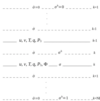
The GLOBO prognostic variables are computed on a Lorenz (1960) vertical grid: all the quantities are on “integer” lev-elsσi, except vertical velocity, turbulent kinetic energy and
mixing length and, consequently, diffusion coefficients, lo-cated at “semi-integer” levelsσih(see Fig. 1). In typical ap-plications, the GLOBO vertical grid is regularly spaced in σ (Malguzzi et al., 2011), although it is possible to use a variable grid spacing, as in its limited-area version BOLAM (Buzzi et al., 1994).
2184 D. Rossi and A. Maurizi: IL-GLOBO: vertical diffusion module
4 Rossi and Maurizi: IL-GLOBO: vertical diffusion module
Fig. 1. Schematic representation of field value distributions be-tween integer (continuous lines) and semi integer (dashed lines) lev-els in the GLOBO model.
for the first order derivative. Following the same consider-ations made forρ, the derivatives ofσwith respect ofzare computed from relationships similar to Eq. (13) and Eq. (14). 255
For the highly varyingKprofiles, two different methods are tested, the first with two variants. The first method in-terpolates the function linearly at the particle position, and uses finite differences derivatives. In the first variant (labeled D), the first order two-points derivative is computed and kept 260
constant between two grid points. In order to give a smoother description of the derivatives, a variant (labeled D′) is also tested in which the three-points centered derivative is com-puted and interpolated linearly at the particle position. For D′
, the values of first order derivative at the lowest boundary 265
is computed as:
∂K ∂σ
NLEV+1
=KNLEV+1−KNLEV
σNLEV+1−σNLEV
. (15)
This is assumed becauseK is expected to be linear near the surface, according to Monin-Obukhov similarity theory where:
270
K(z) =κu∗z, (16)
for the neutral case, with proper modifications for diabatic cases.
The second method (labeled A) is based on the Akima (1991) cubic spline. For each interval it considers the pre-275
vious and the next two adjacent intervals (for a total number of 6 grid points) to compute the coefficients of the interpo-lating cubic polynomial. This algorithm reduces the number of oscillations in the interpolating function compared to reg-ular cubic splines and enforces the linearity when 4 points 280
are collinear (Akima, 1991). Using this property, a linear profile near the ground is imposed to the interpolating func-tion by adding two fictitious points below the ground that are collinear with the two lower grid points of the domain. In ad-dition, to ensure the positivity of the interpolating functions, 285
the local algorithm of Fischer et al. (1991) is used, which also preserves the continuity of first order derivatives.
3.3 Integration scheme and time-step selection
The most common integration scheme for SDE in atmo-spheric transport models is the Euler-Maruyama forward 290
scheme:
Σt+∆t= Σt+a∆t+b∆W . (17)
The coefficients a andbcome from Equation (12). The Euler-Maruyama forward scheme is the simplest strong Tay-lor approximation and turns out to be of order of strong con-295
vergenceγ= 0.5(Kloeden and Platen, 1992, p. 305). By a rather simple modification of the Euler-Maruyama scheme,i.e.adding the term:
1 2bb
′
(∆W2−∆t), (18)
whereb′
is the first-order derivative ofb, the Milstein scheme 300
is obtained, which is of order of strong convergenceγ= 1. It is worth noting that the strong orderγ= 1of the Milstein scheme corresponds to the strong orderγ= 1of the Euler de-terministic scheme. Therefore, Milstein can be regarded as the correct generalization of the deterministic Euler scheme 305
(Kloeden and Platen, 1992, p. 345). The additional term uses only already computed quantities involved in the deter-mination of the drift term of Equation (12). Preliminary ide-alized tests do not show any appreciable accuracy improve-ment with respect to the Euler-Maruyama scheme. However, 310
because they confirm the negligible extra computational cost of this method, the Milnstein scheme will be used to integrate the model.
In the meteorology component of IL-GLOBO, the Eule-rian equations are solved with a macro time-step∆T, which 315
depends basically on the horizontal resolution due to the limitations imposed by the Courant number. Other time-steps are involved in the Eulerian part but are not relevant here. In typical implementations,∆Tranges from 432 s for 362×242point resolution (used for monthly forecasts1) to 320
150 s for1202×818point resolution (used for high resolu-tion weather forecasts2). The macro time-step is taken as the
upper limit for the solution of Equation (12). The time-step needed to reach the required accuracy depends on the quan-tities involved in determining the various elements in Equa-325
tion (17).
1http://www.isac.cnr.it/dinamica/projects/forecast dpc/month
2http://www.isac.cnr.it/dinamica/projects/forecasts/glob
Figure 1. Schematic representation of field value distributions
be-tween integer (continuous lines) and semi-integer (dashed lines) levels in the GLOBO model.
6 being a continuous coordinate, the quantities needed to compute the terms of Eq. (12) must be interpolated from the Eulerian fields given at discrete levels. The computation of first- and second-order derivatives of Eulerian model quan-tities is also required in the implementation of the LSM. In-terpolation and derivation algorithms can influence both the accuracy and the computational cost of the Lagrangian model and thus require careful assessment.
For densityρand geopotential8, linear interpolation and central differences derivative are used assuming that those fields are regular enough. At the lower boundary, it is re-quired that
∂2ρ ∂σ2
NLEV+1
= ∂
2ρ ∂σ2
NLEV
, (13)
which implies ∂ρ
∂σ NLEV+1
= (14)
∂ρ ∂σ
NLEV
+ ∂
2ρ ∂σ2
NLEV
(σNLEV+1−σNLEV)
for the first-order derivative. Following the same considera-tions made forρ, the derivatives ofσ with respect ofzare computed from relationships similar to Eqs. (13) and (14).
For the highly varyingK profiles, two different methods are tested, the first with two variants. The first method in-terpolates the function linearly at the particle position and uses finite differences derivatives. In the first variant (la-belled D), the first-order two-point derivative is computed and kept constant between two grid points. In order to give a smoother description of the derivatives, a variant (labelled D0) is also tested in which the three-point centered derivative is computed and interpolated linearly at the particle position.
For D0, the values of the first-order derivative at the lowest boundary are computed as
∂K ∂σ
NLEV+1
=KNLEV+1−KNLEV
σNLEV+1−σNLEV
. (15)
This is assumed because K is expected to be linear near the surface, according to Monin–Obukhov similarity theory where
K(z)=κu∗z (16)
for the neutral case, with proper modifications for diabatic cases.
The second method (labelled A) is based on the Akima (1991) cubic spline. For each interval it considers the previ-ous and the next two adjacent intervals (for a total number of six grid points) to compute the coefficients of the interpolat-ing cubic polynomial. This algorithm reduces the number of oscillations in the interpolating function compared to regular cubic splines and enforces the linearity when four points are collinear (Akima, 1991). Using this property, a linear pro-file near the ground is imposed to the interpolating function by adding two fictitious points below the ground that are collinear with the two lower grid points of the domain. In ad-dition, to ensure the positivity of the interpolating functions, the local algorithm of Fischer et al. (1991) is used, which also preserves the continuity of first-order derivatives.
3.3 Integration scheme and time-step selection
The most common integration scheme for SDE in atmo-spheric transport models is the Euler–Maruyama forward scheme:
6t+1t=6t+a1t+b1W . (17)
The coefficientsa and b come from Eq. (12). The Euler– Maruyama forward scheme is the simplest strong Taylor ap-proximation and turns out to be of the order of strong con-vergenceγ=0.5 (Kloeden and Platen, 1992, p. 305).
By a rather simple modification of the Euler–Maruyama scheme, i.e. adding the term:
1 2bb
0(1W2−1t ) , (18)
D. Rossi and A. Maurizi: IL-GLOBO: vertical diffusion module 2185
because they confirm the negligible extra computational cost of this method, the Milstein scheme will be used to integrate the model.
In the meteorology component of IL-GLOBO, the Eule-rian equations are solved with a macro time step1T, which depends basically on the horizontal resolution due to the lim-itations imposed by the Courant number. Other time steps are involved in the Eulerian part but are not relevant here. In typ-ical implementations, 1T ranges from 432 s for 362×242 point resolution (used for monthly forecasts1) to 150 s for 1202×818 point resolution (used for high-resolution weather forecasts2). The macro time step is taken as the upper limit for the solution of Eq. (12). The time step needed to reach the required accuracy depends on the quantities involved in determining the various elements in Eq. (17).
First, a straightforward constraint is that the time step must satisfy the relationship
p
2K1t1K
∂K
∂σ
−1
, (19)
(Wilson and Yee, 2007, see, e.g.), which expresses the re-quirement that the average root mean square step length must be much smaller than the scale of the variations ofK. This gives rise to a limitation that is consistent with the surface-layer behaviour of the diffusion coefficient, Eq. (16). The condition expressed by Eq. (19) makes1t1vanish forz→0. Such behaviour ensures that the WMC is satisfied theoret-ically, but clearly poses problems for numerical implemen-tation (Ermak and Nasstrom, 2000; Wilson and Yee, 2007). However, in the application of a global model, where parti-cles can be distributed throughout the troposphere, this prob-lem affects only a small fraction of particles in the vicinity of the surface. Therefore, it can be dealt with by selecting a 1tminsmall enough for the solution to be within the accepted error and, at the same time, large enough to not impact the overall computational cost.
In addition to Eq. (19), another constraint is needed to ac-count also for the presence of maxima in theKprofile, which must be present if one considers the whole atmosphere. At maxima (or minima), Eq. (19) gives an unlimited1t1, which is not suitable for the integration of the model as it could cause the trajectory to cross the maximum (or minimum), with a significant change in K(z)associated to a change in ∂zK sign. To avoid this problem, a further constraint is
in-troduced, based on the normalised second-order derivative, which gives an estimation of the width of the maximum. The constraint reads
2K1t2K
∂2K ∂σ2
−1
. (20)
1http://www.isac.cnr.it/dinamica/projects/forecast_dpc/month_
en.htm
2http://www.isac.cnr.it/dinamica/projects/forecasts/glob_
newNH/
The above equation has the property of limiting1t2 accord-ing to the sharpness of theKpeak.
Taking the minimum among1T,1t1and1t2(and replac-ingwith=CT in Eqs. 19 and 20), gives
1t=min "
1T ,CT 2 K
∂K ∂σ
−2 ,CT
2
∂2K ∂σ2
−1#
, (21) where the parameterCT quantifies the “much less” condition
and, therefore, must be at least 0.1 or smaller.
Figure 2 shows the application of Eq. (21) for aKprofile representative of GLOBO (see Sect. 4) and aCT =0.01. The
1t decreases in the presence ofK gradients thanks to con-dition (19), and is limited around theK maximum (where ∂K/∂σ=0) by condition (20). The maximum of1t=1T is attained at higher levels.
It should be kept in mind that the method is based on local quantities and may fail if strong variations ofKoccur in one time step along the particle path. To overcome this problem, an additional constraint is used to make the algorithm non-local (or “less non-local”). Using the1t0computed at the particle position at timet, two other time steps (1t+and1t−) are evaluated at the positions:
6±=6t+a1t0±b1t01/2. (22) The minimum1t among1t0,1t+and1t−is then used to advance the particle position6t+1t.
3.4 Boundary conditions
The necessary boundary condition for the conservation of the probability (and therefore of the mass) is the reflective boundary (Gardiner, 1990, p. 121). Wilson and Flesch (1993) show that the elastic reflection ensures the WMC if the inte-gration time step is small enough. However, in cases of non-homogeneousK, numerical implementation requires that1t vanishes as the particle approaches the boundary. For models that focus on near-surface dispersion, the time step needed to achieve the required accuracy can become very small. Ermak and Nasstrom (2000) describe a theoretically well-founded method to speed up (roughly by a factor of 10) simulations of this kind.
In the case of IL-GLOBO, it will be shown that the elas-tic reflection condition atσ=1, coupled with the adaptive time-step algorithm described in Sect. 3.3, can ensure a good approximation of the solution while maintaining affordable the computational cost.
4 Model verification: the well-mixed condition
In order to verify the vertical diffusion module of IL-GLOBO, a series of experiments was performed with a 1-D version of the code and then tested in a preliminary version of the full 3-D model. Input profiles were obtained by run-ning the low-resolution version of GLOBO (horizontal grid
2186 D. Rossi and A. Maurizi: IL-GLOBO: vertical diffusion module Rossi and Maurizi: IL-GLOBO: vertical diffusion module 5
First, a straightforward constraint is that the time-step must satisfy the relationship
p
2K∆t1≪K ∂K ∂σ −1 , (19)
(see,e.g., Wilson and Yee, 2007), which expresses the
re-330
quirement that the average root-mean square step length must be much smaller than the scale of the variations ofK. This gives rise to a limitation that is consistent with the surface layer behavior of the diffusion coefficient, Eq. (16). The condition expressed by Equation (19) makes∆t1vanish for 335
z→0. Such behavior ensures the WMC is satisfied theoret-ically, but clearly poses problems for numerical implemen-tation (Ermak and Nasstrom, 2000; Wilson and Yee, 2007). However, in the application of a global model, where parti-cles can be distributed throughout the troposphere, this
prob-340
lem affects only a small fraction of particles in the vicinity of the surface. Therefore, it can be dealt with by selecting a∆tmin small enough for the solution to be within the ac-cepted error and, at the same time, large enough to not impact on the overall computational cost.
345
In addition to Equation (19), another constraint is needed to account also for the presence of maxima in theK pro-file, which must be present if one considers the whole at-mosphere. At maxima (or minima), Equation (19) gives an unlimited∆t1, which is not suitable for the integration of the 350
model as it could cause the trajectory to cross the maximum (or minimum), with a significant change inK(z)associated to a change in∂zKsign. To avoid this problem, a further
constraint is introduced, based on the normalized second-order derivative, which gives an estimation of the width of
355
the maximum. The constraint reads:
2K∆t2≪K
∂2K ∂σ2 −1 . (20)
The above Equation has the property of limiting∆t2
accord-ing to the sharpness of theKpeak.
Taking the minimum among∆T,∆t1and∆t2 (and re-360
placing “≪” by “=CT” in Equations (19) and (20)), gives:
∆t= min "
∆T,CT 2 K
∂K
∂σ −2
,CT 2
∂2K ∂σ2
−1#
, (21)
where the parameterCTquantifies the “much less” condition
and, therefore, must be than at least 0.1 or smaller.
Figure 2 shows the application of Eq. (21) for aKprofile
365
representative of GLOBO (see Section 4) and aCT= 0.01.
The∆tdecreases in the presence ofKgradients thanks to condition (19), and is limited around theKmaximum (where ∂K/∂σ= 0) by condition (20). The maximum of∆t= ∆T is attained at higher levels.
370
It should be beared in mind that the method is based on local quantities and may fail in case strong variations ofK occur in one time step along the particle path. To overcome
0.01 0.1 1 10 100
0.6 0.65 0.7 0.75 0.8 0.85 0.9 0.95 1 0 10 20 30 40 50 60 70 80 90 ∆ t [s] K [m 2/s] σ
Fig. 2.Values of integration time-step∆tfor the diffusivity profile shown by the red curve. The green line shows the contribution of Eq. (19), the blue line the contribution of Eq. (20), and the black line
the combined condition (Eq. 21, with∆T= 432sandCT= 0.01).
the problem, an additional constraint is used to make the al-gorithm non-local (orless local). Using the∆t0computed at 375
the particle position at timet, two other time-step (∆t+and
∆t−) are evaluated at the positions:
Σ±= Σt+a∆t0±b∆t10/2. (22)
The minimum∆tamong∆t0,∆t+and∆t−is then used to
advance the particle positionΣt+∆t.
380
3.4 Boundary conditions
The necessary boundary condition for the conservation of the probability (and therefore of the mass) is the reflective boundary (Gardiner, 1990, p. 121). Wilson and Flesch (1993) show that the elastic reflection ensures the WMC if
385
the integration time-step is small enough. However, in cases of non-homogeneousK, numerical implementation requires that∆tvanishes as the particle approaches the boundary. For models that focus on near surface dispersion, the time-step needed to achieve the required accuracy can become very
390
small. Ermak and Nasstrom (2000) describe a theoretically well founded method to speed-up (roughly by a factor of 10) simulations of this kind.
In the case of IL-GLOBO, it will be shown that the elastic reflection condition atσ= 1, coupled with the adaptive time
395
step algorithm described in Section 3.3, can ensure a good approximation of the solution while maintaining affordable the computational cost.
4 Model verification: the well-mixed condition
In order to verify the vertical diffusion module of
IL-400
GLOBO, a series of experiments was performed with a 1-D version of the code and then tested in a preliminary version Figure 2. Values of integration time step1tfor the diffusivity pro-file shown by the red curve. The green line shows the contribution of Eq. (19), the blue line the contribution of Eq. (20) and the black line the combined condition (Eq. 21, with1T =432sandCT =0.01).
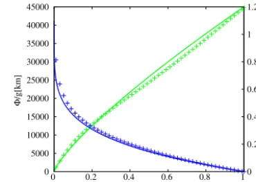
of 362×242 cells and 50 vertical levels evenly spaced inσ) starting at 11 March 2011 00:00 UTC. After 36 h of simula-tion (12:00 UTC), averaging ofσ =const surfaces were per-formed forK,ρand8, obtaining vertical profiles as a func-tion of σ. Fields ofρand8were averaged over the whole domain. As far asKis concerned, averages were performed for latitudes between+60 and−60◦North in daytime (lon-gitudes between−45 and+45◦East) and night-time (longi-tudes between+135 and−135◦East) conditions, over land and sea separately. The most intense K profile is selected which corresponds to the daytime conditions over land. Pro-files ofρandzare rather smooth and regular over space and time, while K displays large variability. The profiles were fitted with analytical functions derived by combining the hy-drostatic equation and the perfect gas law. The following an-alytical expressions were used:
ρ(σ )=ρ0σ(Rd0/g+1), (23)
and z(σ )=(σ
−Rd0/g−1)T0
0 , (24)
with T0=288.0 K, ρ0=1.2 kg m−3 and 0= −0.007 K m−1. As a consequence of the hydrostatic perfect gas assumption, by expressing the densityρin sigma vertical units ρσ=ρ
dz dσ
and using Eqs. (24) and (23), the following constant value is obtained:
ρσ=
ρ0RdT0
g . (25)
Figure 3 shows the GLOBO-average profiles and their fitting functions for the densityρand the geopotential height8g−1 as function ofσ.
As far as theKprofile is concerned, the function
K(z)=Azexph−(Bz)Ci, (26)
6 Rossi and Maurizi: IL-GLOBO: vertical diffusion module
0 5000 10000 15000 20000 25000 30000 35000 40000 45000
0 0.2 0.4 0.6 0.8 1 0 0.2 0.4 0.6 0.8 1 1.2 Φ /g [km] ρ [kg/m 3] σ
Fig. 3. Average GLOBO profiles ofρ(green symbols) andφ/g
(blue symbols) as a function of vertical coordinateσ, and their
ana-lytical fits (Eq. 23 and Eq. 24, lines of the same colors).
of the full 3-D model. Input profiles were obtained by run-ning the low-resolution version of GLOBO (horizontal grid of362×242cells and 50 vertical levels evenly spaced inσ) 405
starting at 2011-03-11 00:00 UTC. After 36 hours of simula-tion (12:00 UTC), averages onσ=const surfaces were per-formed forK,ρandΦ, obtaining vertical profiles as a func-tion ofσ. Fields ofρandΦwere averaged over the whole domain. As far asKis concerned, averages were performed 410
for latitude between +60◦ and -60◦
North in daytime (longi-tude between -45◦
and +45◦
East) and nighttime (longitude between +135◦
and -135◦
East) conditions, over land and sea separately. The most intenseKprofile is selected, which corresponds to the daytime conditions over land. Profiles of 415
ρandzare rather smooth and regular over space and time, whileKdisplays a large variability. The profiles were fitted with analytical functions derived combining the hydrostatic equation and the perfect gas law. The following analytical expressions were used:
420
ρ(σ) =ρ0σ(RdΓ/g+1), (23)
and:
z(σ) =(σ −RdΓ/g
−1)T0
Γ , (24)
withT0= 288.0K,ρ0= 1.2kgm−3andΓ =−0.007K m
−1 . As a consequence of the hydrostatic perfect gas assump-425
tion, by expressing the density ρ in sigma vertical units (ρσ=ρ
ddzσ
) and using Equations (24) and (23), the follow-ing constant value is obtained:
ρσ=
ρ0RdT0
g . (25)
Figure 3 shows the GLOBO averaged profiles and their fit-430
ting functions for the densityρand the geopotential height Φg−1as function ofσ.
0 10 20 30 40 50 60 70 80 90
0.6 0.65 0.7 0.75 0.8 0.85 0.9 0.95 1
K [m
2/s]
σ
Fig. 4. Diffusivity profiles used in the experiments. The symbols represents the data from GLOBO and the lines their fitting function. The ‘average’ profile is shown in red, while the ‘peaked’ profile is shown in green. The functional form of both profiles is described by Eq. (26).
As far as theKprofile is concerned, the function
K(z) =Azexp
−(Bz)C
, (26)
is used to account for the specificKfeatures: it should dis-435
play a linear behavior near the surface, must tend to zero near the boundary layer top3and, therefore, must display a
maximum at some height. In Equation (26),A= 0.29ms−1 was first determined according to average surface-layer prop-erties (the first GLOBO vertical level), and corresponds to 440
a friction velocityu∗≃0.7ms −1
. Then, the other two pa-rameters were let to vary to fit the average profile giving B = 1.3×10⁻³
m−1
andC = 1.6.
Although the above profile is representative of the typi-cal GLOBO diffusivity, real profiles can be remarkably less 445
regular, creating challenging conditions for the model. For this reason, a profile was selected among those showing iso-lated strong maximum near the ground. This is typical of strong convective conditions just after sunrise. Fitting Equa-tion (26) on this second profile gives A= 0.3ms−1,B=
450
4.0×10⁻³
m−1andC= 4.5. Figure 4 reports the GLOBO ‘averaged’ and ‘peaked’Kprofiles as function ofσ.
4.1 Determination of the optimal setting for the adap-tive time-step selection algorithm
The first series of experiments concerns the optimization of 455
the adaptive scheme for∆t,i.e., the selection of the best suited value for the coefficientCTin Equation 21.
Simulations were performed in flow conditions described by Equations (23), (24) and (26), distributing particles with number concentration proportional toρ. For the WMC to be 460
3In GLOBO,Kalso accounts for a part of the instability
gen-erated by moist convection and therefore it may not vanish at the boundary layer top.
Figure 3. Average GLOBO profiles ofρ(green symbols) andφ/g
(blue symbols) as a function of vertical coordinateσand their ana-lytical fits (Eqs. 23 and 24).
Table 1. RMSE and execution time for differentCT.
CT RMSE Time [s]
0.5 0.044 76
0.1 0.037 238
0.01 0.021 1172
0.001 0.021 7317
is used to account for the specificK features: it should dis-play a linear behaviour near the surface, must tend to zero near the boundary layer top3and, therefore, must display a maximum at some height. In Eq. (26),A=0.29 ms−1 was first determined according to average surface-layer proper-ties (the first GLOBO vertical level), and corresponds to a friction velocityu∗'0.7 ms−1. Then, the other two param-eters were allowed to vary to fit the average profile giving B=1.3×10⁻³m−1andC=1.6.
Although the above profile is representative of the typi-cal GLOBO diffusivity, real profiles can be remarkably less regular, creating challenging conditions for the model. For this reason, a profile was selected among those showing iso-lated strong maxima near the ground. This is typical of strong convective conditions just after sunrise. Fitting Eq. (26) to this second profile givesA=0.3 ms−1,B=4.0×10⁻³m−1 andC=4.5. Figure 4 reports the GLOBO “average” and “peaked”Kprofiles as function ofσ.
4.1 Determination of the optimal setting for the adaptive time-step selection algorithm
The first series of experiments concerns the optimisation of the adaptive scheme for 1t, i.e. the selection of the best suited value for the coefficientCT in Eq. (21).
3In GLOBO,Kalso accounts for a part of the instability
D. Rossi and A. Maurizi: IL-GLOBO: vertical diffusion module 2187
6 Rossi and Maurizi: IL-GLOBO: vertical diffusion module
0 5000 10000 15000 20000 25000 30000 35000 40000 45000
0 0.2 0.4 0.6 0.8 1 0 0.2 0.4 0.6 0.8 1 1.2 Φ /g [km] ρ [kg/m 3] σ
Fig. 3. Average GLOBO profiles ofρ(green symbols) andφ/g
(blue symbols) as a function of vertical coordinateσ, and their
ana-lytical fits (Eq. 23 and Eq. 24, lines of the same colors).
of the full 3-D model. Input profiles were obtained by run-ning the low-resolution version of GLOBO (horizontal grid of362×242cells and 50 vertical levels evenly spaced inσ) 405
starting at 2011-03-11 00:00 UTC. After 36 hours of simula-tion (12:00 UTC), averages onσ=const surfaces were per-formed forK,ρandΦ, obtaining vertical profiles as a func-tion ofσ. Fields ofρandΦwere averaged over the whole domain. As far asKis concerned, averages were performed 410
for latitude between +60◦ and -60◦
North in daytime (longi-tude between -45◦and +45◦East) and nighttime (longitude between +135◦
and -135◦
East) conditions, over land and sea separately. The most intenseKprofile is selected, which corresponds to the daytime conditions over land. Profiles of 415
ρandzare rather smooth and regular over space and time, whileKdisplays a large variability. The profiles were fitted with analytical functions derived combining the hydrostatic equation and the perfect gas law. The following analytical expressions were used:
420
ρ(σ) =ρ0σ(RdΓ/g+1), (23)
and:
z(σ) =(σ
−RdΓ/g−1)T 0
Γ , (24)
withT0= 288.0K,ρ0= 1.2kgm−3andΓ =−0.007K m−1.
As a consequence of the hydrostatic perfect gas assump-425
tion, by expressing the density ρ in sigma vertical units (ρσ=ρ
ddσz
) and using Equations (24) and (23), the follow-ing constant value is obtained:
ρσ=ρ0RdT0
g . (25)
Figure 3 shows the GLOBO averaged profiles and their fit-430
ting functions for the densityρand the geopotential height Φg−1as function ofσ.
0 10 20 30 40 50 60 70 80 90
0.6 0.65 0.7 0.75 0.8 0.85 0.9 0.95 1
K [m
2/s]
σ
Fig. 4. Diffusivity profiles used in the experiments. The symbols represents the data from GLOBO and the lines their fitting function. The ‘average’ profile is shown in red, while the ‘peaked’ profile is shown in green. The functional form of both profiles is described by Eq. (26).
As far as theKprofile is concerned, the function
K(z) =Azexp
−(Bz)C
, (26)
is used to account for the specificKfeatures: it should dis-435
play a linear behavior near the surface, must tend to zero near the boundary layer top3 and, therefore, must display a
maximum at some height. In Equation (26),A= 0.29ms−1 was first determined according to average surface-layer prop-erties (the first GLOBO vertical level), and corresponds to 440
a friction velocityu∗≃0.7ms−1. Then, the other two pa-rameters were let to vary to fit the average profile giving B= 1.3×10⁻³m−1andC = 1.6.
Although the above profile is representative of the typi-cal GLOBO diffusivity, real profiles can be remarkably less 445
regular, creating challenging conditions for the model. For this reason, a profile was selected among those showing iso-lated strong maximum near the ground. This is typical of strong convective conditions just after sunrise. Fitting Equa-tion (26) on this second profile givesA= 0.3ms−1, B=
450
4.0×10⁻³m−1andC= 4.5. Figure 4 reports the GLOBO
‘averaged’ and ‘peaked’Kprofiles as function ofσ.
4.1 Determination of the optimal setting for the adap-tive time-step selection algorithm
The first series of experiments concerns the optimization of 455
the adaptive scheme for∆t, i.e., the selection of the best suited value for the coefficientCTin Equation 21.
Simulations were performed in flow conditions described by Equations (23), (24) and (26), distributing particles with number concentration proportional toρ. For the WMC to be 460
3
In GLOBO,Kalso accounts for a part of the instability
gen-erated by moist convection and therefore it may not vanish at the boundary layer top.
Figure 4. Diffusivity profiles used in the experiments. The symbols
represents the data from GLOBO and the lines, their fitting function. The “average” profile is shown in red, while the “peaked” profile is shown in green. The functional form of both profiles is described by Eq. (26).
Simulations were performed in flow conditions described by Eqs. (23), (24) and (26), distributing particles with num-ber concentration proportional to ρ. For the WMC to be satisfied, this distribution must remain constant as the time evolves. Equation (12) was integrated for 4×10⁵ particles and for 200 macro time steps, each 432 s long, for a total of T =86 400 s=24 h. The actual time step used is given by Eq. (21) with the additional lower limit1tmin=0.01. Sim-ulations were performed using 12 cores of an Intel Xeon machine. Since the initial condition was already well-mixed (C∝ρ), the simulation time was considered sufficient to as-sess the skill of the model in satisfying the WMC. At the end of the simulation, final concentration profiles were computed in “σ volume”, i.e.c(σ )=N (σ )(1σ )−1, whereN (σ )is the number of particles betweenσ andσ+1σ. The skill of the model in reproducing the WMC was evaluated using the root mean square error (RMSE) of the final normalised concen-tration profile with respect to the normalised density profile (derived using Eq. 25).
Figure 5 reports the different profiles of concentration af-ter 24 h of simulation computed using different values ofCT.
The shaded region represents the interval between 3 standard deviations from the expected value. RMSE values for each simulation are reported in Table 1 along with the computa-tion time. The RMSE error becomes comparable to the sta-tistical error forCT =0.01, which is selected as the optimal
value. In order to evaluate the possible dependency of CT
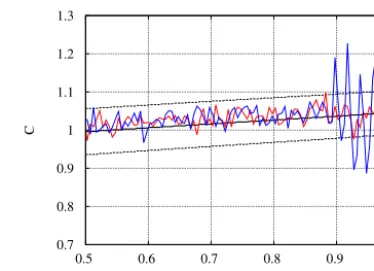
on the number of particles, two additional sets of runs were performed with 105and 16×105particles that correspond to halving and doubling, respectively, the statistical error of the base experiment. Results are reported in Fig. 6 which shows that, in the considered range, the optimalCT is quite
inde-pendent of the number of particles.
It is worth noting that the time-step selection algorithm with the proper choice of CT ensures that the WMC is
also satisfied at the reflective boundary too, as mentioned in Sect. 3.4.
Rossi and Maurizi: IL-GLOBO: vertical diffusion module 7
0.1 1 10 100 1000 0 20 40 60 ∆ t [s] K [m 2/s] 0.8 1 1.2 1.4
0.6 0.65 0.7 0.75 0.8 0.85 0.9 0.95 1
C,
ρnorm
σ
Fig. 5. Dispersion experiment with different choices of parame-terCT. Top panel: diffusivity profile (black line) and∆tprofiles
forCT= 0.5(light blue),CT= 0.1(green),CT= 0.01(red) and
CT= 0.001(blue). Bottom panel: normalized concentration
pro-files for differentCT(Line colors as in the top panel).
satisfied, this distribution must remain constant as the time evolves. Equation (12) was integrated for4×105 particles
and for 200 macro time-steps, each432s long, for a total of T= 86400s= 24h. The actual time-step used is given by Equation (21) with the additional lower limit∆tmin= 0.01.
465
Simulations were performed using 12 cores of an Intel Xeon machine. Since the initial condition was already well-mixed (C∝ρ), the simulation time was considered sufficient to as-sess the skill of the model in satisfying the WMC. At the end of the simulation, final concentration profiles were computed
470
in “σvolume”,i.e.,c(σ) =N(σ)(∆σ)−1, whereN(σ)is the
number of particles betweenσandσ+ ∆σ. The skill of the model in reproducing the WMC was evaluated using the root mean square error (RMSE) of the final normalized concen-tration profile with respect to the normalized density profile
475
(derived using Equation 25).
Figure 5 reports the different profiles of concentration af-ter 24 hours of simulation computed using different values ofCT. The shaded region represents the interval between 3
standard deviations from the expected value. RMSE values
480
for each simulation are reported in Table 1 along with the computation time. The RMSE error becomes comparable to the statistical error forCT= 0.01, which is selected as the
optimal value. In order to evaluate the possible dependency ofCT on the number of particles, two additional sets of runs
485
were performed with105 and16×105particles that
corre-spond to halving and doubling, respectively, the statistical error of the base experiment. Results are reported in Figure 6 which shows that, in the considered range, the optimalCTis
quite independent of the number of particles.
490
It is worth noting that the time-step selection algorithm with the proper choice ofCT ensures that the WMC is also
satisfied at the reflective boundary too, as mentioned in Sec-tion 3.4.
CT RMSE Time [s]
0.5 0.044 76
0.1 0.037 238
0.01 0.021 1172
0.001 0.021 7317
Table 1.RMSE and execution time for differentCT.
0.005 0.01 0.015 0.02 0.025 0.03 0.035 0.04 0.045 0.05
0.001 0.01 0.1
RMSE
CT
Fig. 6. RMSE obtained from experiments made with105
(red),
4×10⁵
(green) and16×105
(blue) particles as a function ofCT.
4.2 Evaluation of the interpolation algorithms
495
In the subsequent set of experiments, the model skill in re-producing the WMC was evaluated for the interpolation tech-niques D, D′
and A described in Section 3.2.
In the first experiment, the analytical fields described by Equations (23), (24) and (26) with the parameters of the
‘av-500
erage’ diffusivity profile were resampled on a 50 point reg-ular grid. This provides a discrete version of the experiment described in the previous section, with the same vertical res-olution of the GLOBO original fields.
The particle number, initial distribution and simulation
505
time are the same as in the experiment described in section 4.1. The integration time-step is selected using the local al-gorithm. The time-step selection algorithm requires the com-putation of the second order derivative ofK, which is not possible for the D interpolation scheme. Therefore, it is
es-510
timated using finite differences of the first order derivative. The results of this experiment are shown in Figure 7. In the upper panel, the integration time-step profiles of the three simulations and the Akima interpolated diffusion coefficient profile, are displayed. The lower panel shows the normalized
515
distribution of the particle after 24 hours of simulation along with the expected value. Table 2 displays the integration time and RMSE obtained for the various experimental settings.
The time-step profiles are similar, except for the A profile around the region of maximum ofK, where it shows strong
520
variations and, on the average, is longer than the others. Looking at the distribution of particles (lower panel), it re-Figure 5. Dispersion experiment with different choices of
param-eterCT. Top panel: diffusivity profile (black line) and1tprofiles forCT =0.5 (light blue),CT =0.1 (green),CT =0.01 (red) and CT =0.001 (blue). Bottom panel: normalised concentration pro-files for differentCT (line colours as in the top panel).
Rossi and Maurizi: IL-GLOBO: vertical diffusion module 7
0.1 1 10 100 1000 0 20 40 60 ∆ t [s] K [m 2/s] 0.8 1 1.2 1.4
0.6 0.65 0.7 0.75 0.8 0.85 0.9 0.95 1
C,
ρnorm
σ
Fig. 5. Dispersion experiment with different choices of parame-terCT. Top panel: diffusivity profile (black line) and∆tprofiles
forCT= 0.5(light blue),CT= 0.1(green),CT= 0.01(red) and
CT= 0.001(blue). Bottom panel: normalized concentration
pro-files for differentCT(Line colors as in the top panel).
satisfied, this distribution must remain constant as the time evolves. Equation (12) was integrated for4×105 particles
and for 200 macro time-steps, each432s long, for a total of T= 86400s= 24h. The actual time-step used is given by Equation (21) with the additional lower limit∆tmin= 0.01.
465
Simulations were performed using 12 cores of an Intel Xeon machine. Since the initial condition was already well-mixed (C∝ρ), the simulation time was considered sufficient to as-sess the skill of the model in satisfying the WMC. At the end of the simulation, final concentration profiles were computed
470
in “σvolume”,i.e.,c(σ) =N(σ)(∆σ)−1, whereN(σ)is the
number of particles betweenσandσ+ ∆σ. The skill of the model in reproducing the WMC was evaluated using the root mean square error (RMSE) of the final normalized concen-tration profile with respect to the normalized density profile
475
(derived using Equation 25).
Figure 5 reports the different profiles of concentration af-ter 24 hours of simulation computed using different values ofCT. The shaded region represents the interval between 3
standard deviations from the expected value. RMSE values
480
for each simulation are reported in Table 1 along with the computation time. The RMSE error becomes comparable to the statistical error forCT = 0.01, which is selected as the
optimal value. In order to evaluate the possible dependency ofCT on the number of particles, two additional sets of runs
485
were performed with105and16×105particles that
corre-spond to halving and doubling, respectively, the statistical error of the base experiment. Results are reported in Figure 6 which shows that, in the considered range, the optimalCT is
quite independent of the number of particles.
490
It is worth noting that the time-step selection algorithm with the proper choice ofCT ensures that the WMC is also
satisfied at the reflective boundary too, as mentioned in Sec-tion 3.4.
CT RMSE Time [s]
0.5 0.044 76
0.1 0.037 238
0.01 0.021 1172
0.001 0.021 7317
Table 1.RMSE and execution time for differentCT.
0.005 0.01 0.015 0.02 0.025 0.03 0.035 0.04 0.045 0.05
0.001 0.01 0.1
RMSE
CT
Fig. 6. RMSE obtained from experiments made with105
(red),
4×10⁵
(green) and16×105
(blue) particles as a function ofCT.
4.2 Evaluation of the interpolation algorithms
495
In the subsequent set of experiments, the model skill in re-producing the WMC was evaluated for the interpolation tech-niques D, D′
and A described in Section 3.2.
In the first experiment, the analytical fields described by Equations (23), (24) and (26) with the parameters of the
‘av-500
erage’ diffusivity profile were resampled on a 50 point reg-ular grid. This provides a discrete version of the experiment described in the previous section, with the same vertical res-olution of the GLOBO original fields.
The particle number, initial distribution and simulation
505
time are the same as in the experiment described in section 4.1. The integration time-step is selected using the local al-gorithm. The time-step selection algorithm requires the com-putation of the second order derivative ofK, which is not possible for the D interpolation scheme. Therefore, it is
es-510
timated using finite differences of the first order derivative. The results of this experiment are shown in Figure 7. In the upper panel, the integration time-step profiles of the three simulations and the Akima interpolated diffusion coefficient profile, are displayed. The lower panel shows the normalized
515
distribution of the particle after 24 hours of simulation along with the expected value. Table 2 displays the integration time and RMSE obtained for the various experimental settings.
The time-step profiles are similar, except for the A profile around the region of maximum ofK, where it shows strong
520
variations and, on the average, is longer than the others. Looking at the distribution of particles (lower panel), it re-Figure 6. RMSE obtained from experiments made with 105(red), 4×10⁵(green) and 16×105(blue) particles as a function ofCT.
4.2 Evaluation of the interpolation algorithms
In the subsequent set of experiments, the model skill in re-producing the WMC was evaluated for the interpolation tech-niques D, D0and A described in Sect. 3.2.
In the first experiment, the analytical fields described by Eqs. (23), (24) and (26) with the parameters of the “average” diffusivity profile were resampled on a 50-point regular grid. This provides a discrete version of the experiment described in the previous section, with the same vertical resolution of the GLOBO original fields.
The particle number, initial distribution and simulation time are the same as in the experiment described in Sect. 4.1. The integration time step is selected using the local algo-rithm. The time-step selection algorithm requires the com-putation of the second-order derivative ofK, which is not possible for the D interpolation scheme. Therefore, it is es-timated using finite differences of the first-order derivative. The results of this experiment are shown in Fig. 7. In the upper panel, the integration time-step profiles of the three simulations and the Akima interpolated diffusion coefficient profile are displayed. The lower panel shows the normalised
2188 D. Rossi and A. Maurizi: IL-GLOBO: vertical diffusion module
Table 2. Execution time and RMSE for experiments made with the
sampled “average” diffusivity distribution and varying interpolation method.
Interpolation algorithm Exec. time RMSE
A 237 s 0.025
D 155 s 0.023
D0 162 s 0.044
8 Rossi and Maurizi: IL-GLOBO: vertical diffusion module
0.1 1 10 100 1000 0 20 40 60 80 ∆ t [s] K [m 2/s] 0.8 1 1.2 1.4
0.6 0.65 0.7 0.75 0.8 0.85 0.9 0.95 1
C,
ρnorm
σ
Fig. 7. Experiments with the sampled ‘average’ diffusivity distri-bution for the interpolation algorithms D (blue), D′(green) and A
(red). Top panel: Diffusivity profile as interpolated by A (black) and
∆tprofiles for the different interpolation settings. Bottom panel: Normalized final concentration and expected distribution (black).
Interpolation algorithm exec. time RMSE
A 237 s 0.025
D 155 s 0.023
D′ 162 s 0.044
Table 2. Execution time and RMSE for experiments made with the sampled ‘averaged’ diffusivity distribution, varying interpola-tion method.
sults that simulations with A and D interpolation algorithms both satisfy the WMC within the statistical limit, while the simulation with the D′
algorithm fails to maintain the well
525
mixed state, in particular near the ground. Additional ex-periments (not reported) show that in order to obtain a well mixed solution with D′
, resolution must be doubled, at least. The problem is probably related to the definition of deriva-tives ofKbetween grid points. In fact, although D′computes
530
derivatives at higher order of approximation than D, they are not consistent with a linear variation ofK. Although the use of D′
can be appropriate for slowly varying and monotone functions likeρandz, it turns out to be unsuitable for the more complexKprofile which, in addition, affects both the
535
Wiener stochastic term and the drift term. For these reasons, the D′
interpolation scheme is not used in the following ex-periments.
The second experiment concerns the ‘peaked’ profile. In this case, theK profile is used directly, without the
resam-540
pling of the fitting function. Simulations with A and D algo-rithms were performed with both local and non-local time-step selection algorithm. Figure 8 reports the time-time-step and concentration profiles, while execution times and RMSEs are shown in Table 3. Although the integration time-step profiles
545
look very similar for the local and non-local algorithms, the small differences have large impact on the results: the local
Interpolation algorithm ∆tselection exec. time RMSE
A local 313 s 0.042
D local 181 s 0.065
A non-local 1122 s 0.016
D non-local 593 s 0.022
Table 3.Execution time and RMSE for experiments made with the ‘peaked’ diffusivity distribution, varying interpolation method and
∆tselection algorithm.
0.1 1 10 100 1000 ∆ t [s] 0 20 40 K [m 2/s] 0.8 1 1.2
0.9 0.95 1.0
C,
ρnorm
σ
0.9 0.95 1.0
σ
Fig. 8.Same as in Fig. 7 for experiments with the ‘peaked’ diffusiv-ity distribution. Results obtained using the local (left) or non-local (right)∆tselection algorithm.
interpolation schemes, especially for D. Conversely, the non-local algorithm turns out to be effective in selecting the
ap-550
propriate time-step even in presence of strong gradients and isolated maxima. This is reflected on its higher computa-tional cost (see Table 3).
4.3 Implementation on the 3-D model
A preliminary test of the algorithms on the 3-D model has
555
been performed. The interpolation algorithm has been imple-mented in a simplified quasi-1-D form, where the diffusion coefficient has been considered to be horizontally constant between grid points. IL-GLOBO uses the same paralleliza-tion of GLOBO, with particle exchanged between processes
560
at each macro time-step. Particles are first advected horizon-tally for a macro time-step using their deterministic velocity, and then ‘diffused’ in the vertical according to Equation (12). After 12 h of spinup,5×105particles are released with a
vertical distribution proportional to the average density
pro-565
file, and randomly and homogeneously distributed in the hor-izontal. Particle statistics are computed after 24 h from the release.
A and D interpolation algorithm were tested using the non-local time-step selection. It is found that, while interpolation
570
scheme A maintains the WMC reasonably (RMSE=0.024), the time-step selection algorithm for scheme D requires ex-Figure 7. Experiments with the sampled “average” diffusivity
dis-tribution for the interpolation algorithms D (blue), D0(green) and A (red). Top panel: diffusivity profile as interpolated by A (black) and
1t profiles for the different interpolation settings. Bottom panel: normalised final concentration and expected distribution (black).
distribution of the particle after 24 h of simulation along with the expected value. Table 2 displays the integration time and RMSE obtained for the various experimental settings.
The time-step profiles are similar, except for the A pro-file around the region of the maximum ofK, where it shows strong variations and, on the average, is longer than the oth-ers. Looking at the distribution of particles (lower panel), it can be observed that simulations with A and D interpolation algorithms both satisfy the WMC within the statistical limit, while the simulation with the D0algorithm fails to maintain the well-mixed state, in particular near the ground. Addi-tional experiments (not reported) show that in order to obtain a well-mixed solution with D0, resolution must be doubled at least. The problem is probably related to the definition of derivatives of K between grid points. In fact, although D0 computes derivatives at a higher order of approximation than D, they are not consistent with a linear variation ofK. Al-though the use of D0 can be appropriate for slowly varying and monotone functions likeρ andz, it turns out to be un-suitable for the more complexK profile which, in addition, affects both the Wiener stochastic term and the drift term. For these reasons, the D0interpolation scheme is not used in the following experiments.
The second experiment concerns the “peaked” profile. In this case, the K profile is used directly, without the re-sampling of the fitting function. Simulations with A and D algorithms were performed with both local and non-local
Table 3. Execution time and RMSE for experiments made with the
“peaked” diffusivity distribution, varying interpolation method and
1tselection algorithm.
Interpolation algorithm 1tselection Exec. time RMSE
A local 313 s 0.042
D local 181 s 0.065
A non-local 1122 s 0.016
D non-local 593 s 0.022
8 Rossi and Maurizi: IL-GLOBO: vertical diffusion module
0.1 1 10 100 1000 0 20 40 60 80 ∆ t [s] K [m 2/s] 0.8 1 1.2 1.4
0.6 0.65 0.7 0.75 0.8 0.85 0.9 0.95 1
C,
ρnorm
σ
Fig. 7. Experiments with the sampled ‘average’ diffusivity distri-bution for the interpolation algorithms D (blue), D′(green) and A
(red). Top panel: Diffusivity profile as interpolated by A (black) and
∆tprofiles for the different interpolation settings. Bottom panel:
Normalized final concentration and expected distribution (black).
Interpolation algorithm exec. time RMSE
A 237 s 0.025
D 155 s 0.023
D′ 162 s 0.044
Table 2. Execution time and RMSE for experiments made with the sampled ‘averaged’ diffusivity distribution, varying interpola-tion method.
sults that simulations with A and D interpolation algorithms both satisfy the WMC within the statistical limit, while the simulation with the D′
algorithm fails to maintain the well
525
mixed state, in particular near the ground. Additional ex-periments (not reported) show that in order to obtain a well mixed solution with D′
, resolution must be doubled, at least. The problem is probably related to the definition of deriva-tives ofKbetween grid points. In fact, although D′
computes
530
derivatives at higher order of approximation than D, they are not consistent with a linear variation ofK. Although the use of D′
can be appropriate for slowly varying and monotone functions likeρandz, it turns out to be unsuitable for the more complexKprofile which, in addition, affects both the
535
Wiener stochastic term and the drift term. For these reasons, the D′interpolation scheme is not used in the following ex-periments.
The second experiment concerns the ‘peaked’ profile. In this case, theK profile is used directly, without the
resam-540
pling of the fitting function. Simulations with A and D algo-rithms were performed with both local and non-local time-step selection algorithm. Figure 8 reports the time-time-step and concentration profiles, while execution times and RMSEs are shown in Table 3. Although the integration time-step profiles
545
look very similar for the local and non-local algorithms, the small differences have large impact on the results: the local algorithm strongly fails in reproducing the WMC for both
Interpolation algorithm ∆tselection exec. time RMSE
A local 313 s 0.042
D local 181 s 0.065
A non-local 1122 s 0.016
D non-local 593 s 0.022
Table 3.Execution time and RMSE for experiments made with the ‘peaked’ diffusivity distribution, varying interpolation method and
∆tselection algorithm.
0.1 1 10 100 1000 ∆ t [s] 0 20 40 K [m 2/s] 0.8 1 1.2
0.9 0.95 1.0
C,
ρnorm
σ
0.9 0.95 1.0
σ
Fig. 8.Same as in Fig. 7 for experiments with the ‘peaked’ diffusiv-ity distribution. Results obtained using the local (left) or non-local (right)∆tselection algorithm.
interpolation schemes, especially for D. Conversely, the non-local algorithm turns out to be effective in selecting the
ap-550
propriate time-step even in presence of strong gradients and isolated maxima. This is reflected on its higher computa-tional cost (see Table 3).
4.3 Implementation on the 3-D model
A preliminary test of the algorithms on the 3-D model has
555
been performed. The interpolation algorithm has been imple-mented in a simplified quasi-1-D form, where the diffusion coefficient has been considered to be horizontally constant between grid points. IL-GLOBO uses the same paralleliza-tion of GLOBO, with particle exchanged between processes
560
at each macro time-step. Particles are first advected horizon-tally for a macro time-step using their deterministic velocity, and then ‘diffused’ in the vertical according to Equation (12). After 12 h of spinup,5×105particles are released with a
vertical distribution proportional to the average density
pro-565
file, and randomly and homogeneously distributed in the hor-izontal. Particle statistics are computed after 24 h from the release.
A and D interpolation algorithm were tested using the non-local time-step selection. It is found that, while interpolation
570
scheme A maintains the WMC reasonably (RMSE=0.024), the time-step selection algorithm for scheme D requires ex-tremely short time-steps (≪∆tmin, see Section 4.1) in the Figure 8. Same as in Fig. 7 for experiments with the “peaked”
dif-fusivity distribution. Results obtained using the local (left) or non-local (right)1tselection algorithm.
time-step selection algorithms. Figure 8 reports the time-step and concentration profiles, while execution times and RM-SEs are shown in Table 3. Although the integration time-step profiles look very similar for the local and non-local al-gorithms, the small differences have a large impact on the results: the local algorithm mostly fails in reproducing the WMC for both interpolation schemes, especially for D. Con-versely, the non-local algorithm turns out to be effective in selecting the appropriate time step, even in the presence of strong gradients and isolated maxima. This is reflected in its higher computational cost (see Table 3).
4.3 Implementation on the 3-D model
A preliminary test of the algorithms on the 3-D model has been performed. The interpolation algorithm has been imple-mented in a simplified quasi-1-D form, where the diffusion coefficient has been considered to be horizontally constant between grid points. IL-GLOBO uses the same parallelisa-tion of GLOBO, with particles exchanged between processes at each macro time step. Particles are first advected horizon-tally for a macro time step using their deterministic velocity and then “diffused” in the vertical according to Eq. (12).