Nonlinear Analysis of Truss Structures Using Dynamic Relaxation (RESEARCH NOTE)

(1)

RESEARCH NOTE

NONLINEAR ANALYSIS OF TRUSS STRUCTURES

USING DYNAMIC RELAXATION

M. Rezaee Pajand* and M. Taghavian Hakkak

Department of Civil Engineering, Ferdowsi University of Mashhad Mashhad, Iran, [email protected]

*Corresponding Author

(Received: September 4, 2005 – Accepted in Revised Form: November 2, 2006)

Abstract This paper presents a new approach for large-deflection analysis of truss structures employing the Dynamic Relaxation method (DR). The typical formulation for DR has been established utilizing the finite difference technique which is categorized as an explicit method. The special characteristic of the explicit method is its simple algebraic relationships in comparison with complicated matrix operations in a finite element method. In this paper, a new procedure is developed using the Taylor series in order to reduce the number of iterations needed for convergence and consequently time and effort. Moreover, the validity of the proposed technique has been demonstrated by solving some truss structures with nonlinear behavior.

Key Words Convergence, Higher Order, Nonlinear Analysis, Dynamic Relaxation, Truss, Large Displacement, Taylor Series

ﻩﺪﻴﮑﭼ

ﯽﻣ ﺎﺟﯽﻨﻤﺿ ﻭﺢﻳﺮﺻﻪﺘﺳﺩ ﻭﺩﺭﺩ ﯽﻄﺧﺮﻴﻏﯼﺎﻫ ﻞﻴﻠﺤﺗ

ﺪﻧﺮﻴﮔ .

ﻩﺩﺎﺳﯼﺎﻫ ﻪﻄﺑﺍﺭﺎﺑﺢﻳﺮﺻ ﺵﻭﺭ

ﺟ

ﯽﻣﻡﺎﺠﻧﺍﯽﺴﻳﺮﺗﺎﻣﺕﺎﻴﻠﻤﻋﺯﺍﯼﺭﻭﺩﻭﯼﺮﺒ

ﺩﺮﻳﺬﭘ .

ﺩﺭﺍﺩﺭﺍﺮﻗ ﻩﻭﺮﮔﻦﻳﺍﺭﺩﺎﻳﻮﭘﯽﻳﺎﻫﺭﺭﺎﮑﻫﺍﺭ

.

ﺩﻭﺪﺤﻣﺕﻭﺎﻔﺗ

ﺖﺳﺍﻩﻮﻴﺷﻦﻳﺍﯼﺯﺎﺳﻪﻄﺑﺍﺭﻩﺍﺭﻦﻳﺮﺘﻧﺎﺳﺁ

.

ﺶﻫﺎﮐﯼﺍﺮﺑﺭﻮﻠﻴﺗﻪﻟﺎﺒﻧﺩﺵﺮﺘﺴﮔﻪﻳﺎﭘﺮﺑﻮﻧﺵﻭﺭﮏﻳ،ﻪﻌﻟﺎﻄﻣﻦﻳﺍﺭﺩ

ﯽﻣ ﺩﺎﻬﻨﺸﻴﭘ ﺎﻫﺭﺍﺮﮑﺗ

ﺩﻮﺷ .

ﯽﻳﺎﭘﺮﺧ ﻩﺯﺎﺳ ﺪﻨﭼ ﯼﺩﺎﻬﻨﺸﻴﭘ ﺭﺎﮑﻫﺍﺭ ﺎﺑ

ﯽﻣ ﻞﻴﻠﺤﺗ

ﻥﺍﺮﮕﻳﺩ ﺭﺎﮐ ﺎﺑ ﺎﻬﻧﺁ ﻪﺠﻴﺘﻧ ﻭﺩﻮﺷ

ﯽﻣﻪﺴﻳﺎﻘﻣ

ﺩﺩﺮﮔ .

1. INTRODUCTION

In order to analyze various engineering problems with geometrical nonlinearity, a stable and efficient numerical method is of great importance. Also, it is essential to develop a powerful algorithm appropriate for a wide range of problems. The newly developed dynamic relaxation method (DRM) has proved to have a promising potential with a number of distinguished features. For instance, it has a clear and simple algorithm so that the required computer programming is straightforward. Moreover, it needs not to solve large scale equations directly, because of its explicit formulation. Finally, it is very reliable and stable for analyzing nonlinear problems.

(2)

mathematical way [1].

As an iterative method, the DR scheme has a corrector procedure. In this approach, the tangent stiffness matrix has a great deal of importance. Moreover, the unbalanced force is used to correct the displacement vector.

In the following, a brief history of dynamic relaxation will be reviewed. Then, the DR method will be presented by illustrating its formulation and suggesting strategies for the determination of its required factors. Finally, a new formulation is introduced and some examples are solved to investigate the capability of the proposed technique.

2. BRIEF HISTORY

Using the Dynamic Relaxation process goes back to the first decades of the twentieth century. This term is an abbreviation of systematic relaxation of constraints. It has an iterative procedure for solving large equation systems making use of finite difference method [2].

In the nineteenth century, Rayleigh presented a new way for the static solution of a mechanic system. He regarded the steady state solution of a dynamic system as a static solution. In 1950, Frankle developed the DR method which originates from the second - order Richardson role [3]. Frankle states that the formal equivalence of Richardson algorithm to the first order time dependant equations suggests the extension to a solution algorithm equivalent to a second order time dependant equation. For this, it seems that Frankle was the first one who made the connection between the static problems and dynamics. The terms of Dynamic Relaxation appears to have been coined by Otter in the mid – 1960s. Cassell [4] and Welsh [5] are among the researchers who developed this method and applied it to the structural analysis. They introduced the artificial mass. Then, Rushton applied the Dynamic Relaxation scheme to the nonlinear analysis of structures [6]. In recent decades, Underwood and Park have conducted numerous researches. Wood worked on explicit formulation and also compared this method with other existing ones [7]. From 1970 till now, a large number of investigations

have been conducted in this field. They have demonstrated that the Dynamic Relaxation technique can be used as a powerful and reliable method for analyzing engineering problems [8, 9]. Its abilities will be more obvious in comparison with other methods.

3. ADVANTAGES AND DISADVANTAGES

In comparison with other methods, the dynamic relaxation scheme has its own strengths and weaknesses. These characteristics

are mentioned

below:

Advantages

• The method has a simple algorithm so that it is will be very convenient for programming.

• The formulation is explicit. Therefore, the required memory is less than other techniques.

• This method has a high ability in intense nonlinear behaviors.

Disadvantages

• In general, the method is unstable and needs some additional conditions to guarantee numerical stability.

• Iterations of the method are done in constant load. This causes some issues in limit points.

• In nonlinear analysis, with gentle stiffening, the number of iterations is much more in comparison with the Newton methods.

4. FORMULATION

(3)

dependant equation. In other words, in the dynamic relaxation method, a static system is transferred to the artificial dynamic space by adding artificial inertia and damping forces as follow:

} ) t ( P { } x ]{ K [ } x { ] C [ } x { ] M

[ && n+ & n+ n = n (1)

In this equation, [M], [C] and [K] are mass, damping, and stiffness matrix, respectively. Also, {x} is the displacement vector and _{_x_&_}n_and_{_x_&&_}n are its first and second rank derivatives which are regarded as velocity and acceleration. Using the finite difference method, the velocity and acceleration vectors can be written as follows:

h } x { } x { } x { 2 1 2 1 _n n

n ₌ & + − & −

&& (2)

h {x} {x} }

x

{_& n-12 = n− n-1 (3)

In these equations, h is the artificial time step. The velocity can also be derived by the following average value: 2 } x { } x { } x { 2 1 2 1 _n -n

n ₌ & + & +

& (4)

By substituting Equations 2 and 4 into 1, an iterative equation for velocity in the )

2 1 (n+ , th step will be obtained. Also, the displacement in the next step, (n + 1) th, will be achieved. These relations are as follows:

) [C]/2 [M]/h ( ) } x ]{ K [ ({p} } x { ) [C]/2 [M]/h ( ) 2 / ] [C h / [M] ( } x

{ n 21 n 21

+ − + + − = − + & & (5) 2 1 n n 1

n _{x} _h{_x_}

{x} + = + & + (6)

In order to have explicit iterative equations, the artificial mass should be considered as a diagonal matrix. Also, the damping matrix will be dependent on the mass matrix in the following form:

] M [ c ] C

[ = (7)

c is the damping coefficient. Substituting Equation 7 into 5, leads to the following iterative relations [9]:

n 1 n

n _[_M_] _.{R}

ch) (2 2h } x .{ ) ch 2 ( ) ch -2 ( } x

{ +21 −21 −

+ + +

= &

& (9)

2 1

n n 1

n _{x} _h{_x_}

{x} + = + & + (10)

Here, {R}n is the residual force vector defined as follow:

[K]{x} {P}

{R}n = n− (11)

The solution can be achieved by applying Equation 9 and 10 and some other appropriate assumptions for coefficient c, the time increment h, and the mass matrix [M]. It is recommended to choose the zero vector for {x}0_and

{ }

2 1

x& − at the beginning of the dynamic relaxation procedure. In this way, the velocity at mid-step will be calculated from 9. Then, the displacement vector in the first step will be found using 10. Subsequently, this procedure will continue until the solution converges on the steady state response. In each step, the displacement and velocity vectors are modified. It is important to choose the artificial mass, damping and time step so that the stability and the fastest convergence rate are obtained. Note that only internal and external forces may represent the physical problem.

5. REQUIRED FACTORS

As mentioned before, in the dynamic relaxation method a static problem must be transferred to a virtual dynamic space in order to find the steady state response. This transference enters some required factors to the problem which is necessary to begin the DR procedure. On the other hand, the dynamic relaxation iterations are generally unstable. Therefore, the required factors must be determined so that the numerical stability guarantees convergence of the procedure. The required factors are as follows:

(4)

• Damping coefficient

• Time step

• The initial displacement vector

Several strategies have been put forward to specify these factors appropriately and also with the aim of accelerating the convergence rate. In the following, some of these strategies will be expounded briefly. It should be noted that all of these factors are fictitious.

5.1. Mass

The first step in the dynamic relaxation process is determination the mass matrix. It must be pointed out that the DR method is a technique to solve the system of equations. In order to preserve the explicit characteristic of the method and avoid extra calculation for inversing the mass matrix, a diagonal mass matrix is considered. Some suggested schemes for the mass matrix are as follows:

5.1.1. Unit matrix In this technique, the mass matrix is considered as the following unit matrix [9].

[ ] [ ]

M =α I (12)

In this equation, α is a real number. Therefore, the mass matrix has the same value with a different degree of freedom. Because of shortcomings, there is not enough accuracy. This escalates the number of iterations. It is not, therefore, usually used.

5.1.2. Mass proportioned with stiffness matrix

Here, diagonal entries of the mass matrix

are proportional to the stiffness matrix as follows [9]:

[ ] [ ]

M =α K (13)

Here again, α is a real number. It is common to consider α = 1. This method has an efficient application in comparison with the unit matrix because the mass matrix has different value in each degree of freedom. For the change of mass value in each iteration according to the stiffness matrix, this approach is very common in nonlinear analysis. It should be noted that this technique does not have a mathematical basis.

5.1.3. The absolute squared value In this scheme, each diagonal element of the mass matrix is formed by summing the absolute squared values of all the entries in the corresponding row of the stiffness matrix [10].

∑ = = q

1

j ij

K ii

m (14)

Where, q demonstrates the number of the degree of freedom. This method increases the calculation operations and requires more memory. However, the mass values almost ensure the stability and convergence acceleration during the procedure of nonlinear analysis. The reason is that each degree of freedom has its own value which is not similar to the others. It must be pointed out that there is no mathematical basis for this scheme too.

5.1.4. Gerschgorin’s theorem Having the mathematical basis, this scheme is the most efficient and applicable one to determine the mass matrix, and has proved its validity to guarantee the stability of the process. The ability of this approach is more obvious in solving nonlinear problems. Physically, this theorem is equivalent to assume the highest eigenvalue vector, that is a subsequence of 1, -1, 1, -1, …. This technique gives the following general expression for the mass values [15]:

∑ =

≥ n

1 j Kij 2

h 4 1 ii

m (15)

5.2. Damping Factor

Another important factor to guarantee the convergence and stability of the analysis procedure is damping. The most effective way employs the critical damping. Many researches have been conducted to find the appropriate value for this parameter and among them; Rayleigh’s theory is the most common way. In the following lines, some prominent techniques are covered.

(5)

determining the mass and assuming a zero value for damping. Then, displacements are found through the iterations. Afterwards, the displacement - time curve will be drawn for this system. Having this diagram, it would be possible to calculate the lowest period of the system [9]. Finally, the damping factor is found from the following relationship:

o 2ω

c= (16)

5.2.2. Underwood suggestion In this scheme, the damping factor is corrected by new - found data which are obtained throughout the procedure. Here again, Rayleigh’s theory is utilized. Note that the damping factor is fixed during the iterations. This value can be calculated as below [11]:

{ }

[ ]

{ }

2 1 x M T x x n K T x 2 n c ⎪ ⎭ ⎪ ⎬ ⎫ ⎪ ⎩ ⎪ ⎨ ⎧ ⎥⎦ ⎤ ⎢⎣ ⎡

= (17)

Where, the mass matrix is formed by Gerschgorin’s theorem. Note that [K___n] is a diagonal matrix and its entries are calculated by:

{

} {

}

2 1 n i 1 n i n i i n x h ) x ( F ) x ( F

K = −₋ −

& (18)

In this equation, Fi shows the internal force of the ith degree of freedom. The value from Equation 17 is an estimate of the critical damping factor which is formed by the tangent stiffness matrix in the last position of the structure. This method has a high ability in nonlinear analysis.

5.2.3. The Zhang suggestion In this approach, the critical damping factor is calculated as follow [12]:

{ }

{

( )

}

{ }

2 1 n X n M T x X n X F T n X 2 n c ⎪ ⎭ ⎪ ⎬ ⎫ ⎪ ⎩ ⎪ ⎨ ⎧ ⎥⎦ ⎤ ⎢⎣ ⎡

= (19)

Here, Rayleigh’s theory is the basis of the

methodology. The advantages of this method are low calculations and low required memory. It is worth mentioning that the damping factor is constant for all degrees of freedom.

5.2.4. The Qiang suggestion In this scheme, the damping factor is obtained by minimizing the displacement error and Rayleigh’s theory. Qiang suggested this parameter as follows [13]:

2 1 o ω 1 o ω 2 n

c _⎟⎟

⎠ ⎞ ⎜ ⎜ ⎝ ⎛ +

= (20)

Where, ωo is the lowest natural period of the system in free vibration and will be calculated by:

{ }

n T

[ ]

n

{ }

n n X M X n x T n K X o ω ⎥⎦ ⎤ ⎢⎣ ⎡

= (21)

In this technique, _⎢⎣⎡KT_n_⎥⎦⎤ demonstrates the tangent stiffness matrix in the nth step, and the mass matrix is calculated by Gerschgorin’s theorem.

5.2.5. Crisfield suggestion Crisfield presented another scheme for estimating this factor based on Rayleigh’s theory [14]:

{ }

{

}

{ }

[ ]

{

}

2 1 n X Δ M T n X Δ n X Δ diag K n X Δ 2 n c ⎪ ⎭ ⎪ ⎬ ⎫ ⎪ ⎩ ⎪ ⎨ ⎧ ⎥⎦ ⎤ ⎢⎣ ⎡

= (22)

In this expression, Δ illustrates the variation from the previous step and [K]diag is a stiffness matrix that is composed of only diagonal entries.

5.3. Time Step

Another parameter that has a

(6)

Some proposed schemes suggested by different researchers are as follows:

5.3.1. Constant time step Using a fixed and constant time increment during the entire iterations is more usual than other ways. In fact, this method is very useful when the aim is the comparison of other factors such as mass and damping. Several approaches have been presented to determine this value. For instance, the equation below gives a suitable time step [11]:

max ω

2

h ≤ (23)

Where, ωmax is the greatest value of the natural period of structure. In addition to Equation 23, Underwood has suggested that the value of 1 and 1.1 for the time step. Actually, using a constant slightly greater than 1 can ensure the stability and convergence.

5.3.2. Qiang suggestion In this method, the time step has been calculated using Rayleigh’s and Gerschgorin’s theoreom. Qiang proposed the time increment as follows [13]:

2 1 ) o ω (1

2 h

+

= (24)

Here, ωo is the lowest natural period of the structure. This method has an effective application in nonlinear problems, as the time increment varies within iterations.

5.4. The Initial Displacement Vector

Another

factor that can influence the convergence rate is the initial displacement vector. In other words, selecting an appropriate value closer to the answer causes the process to converge on the solution with less iteration. It must be pointed out that the dynamic relaxation procedure usually achieves the solution with any initial displacement vector. The zero and unit vector are the most common and convenient amount for this item. Moreover, they could be guessed experimentally if the behavior of structure is predictable.

6. ANALYSIS STEPS

In the DR method, Equations 9 and 10 are used to obtain the static answer for a structure. Selecting the required parameters (mass, damping and time increment) the procedure can be started. These parameters are necessary at the beginning of the analysis.

The residual force and kinematic energy can usually control the iterations. To do so, first a value must be specified for allowable error. Then, during the analysis procedure, the error is continuously compared with its allowable amount. The calculation is finished when the criterion reaches its allowable level. The Kinematic energy is computed as follow:

∑ =

+ = N

1 i

2 ) 2 1 n i x ( E

K & (25)

When the velocity approaches zero, the variation of displacement will also be zero too. In the following lines, the dynamic relaxation algorithm is presented [9]. Here, the unbalanced force (Rn) is selected as a stopping criterion.

• Determine mass, damping, time increment, an allowable value for error and set n = 0

• Assume

{ }

x& −21 as a zero vector.

• Calculate {x}0 or assume zero for it.

• Calculate unbalanced force by

} x { ] K [ } P { } R

{ n = n − .

• If Rn < e go to 8, otherwise continue.

• Calculate the displacement and velocity using Equations 9 and 10, respectively.

• Increase the number of step (n = n + 1) and return to 4

• Print the results.

• stop

7. SUGGESTED FORMULATION

(7)

productive to have a higher order of error in the DR formulation. In this way, the accuracy of the procedure will increase. Subsequently, the solution will be obtained with less iteration. In this paper, a new approach is introduced to formulate the DR process, with the purpose of improving computational time and effort. In this formulation, the first three terms of the Taylor series will be used to raise the error rank. Utilizing the Taylor series, the below expression states displacement vector for the (n + 1) step:

{ }

_x n 2

2 h n x h n x 1 n

x + = + & + && (26)

Equation 26 can be written in the following form:

{ }

_⎥⎦⎤

⎢⎣

⎡ ₋

= Δx n h x n

2 h

2 n

x&& & (27)

{ } { }

n n 1

{ }

n x x

x

Δ = + − (28)

On the other hand, the governing equation for dynamic systems can be written as follow:

[ ]

_M

{ }

_x n₊_[_C_]

{ } { }

_x n ₌ _R n

&

&& (29)

Substituting 27 into 29 leads to the following relationship:

[ ]

{

_Δ_x

}

n _h.

{ }

_x n _[_C_]

{ }

_x n

{ }

_R n

2 h

2

M _⎟⎟+ =

⎠ ⎞ ⎜

⎜ ⎝ ⎛

⎟ ⎠ ⎞ ⎜

⎝

⎛ ₋ _& _&

(30) Equation 30 can be written:

{ }

_x n

[ ]

_M 1

{ }

_R n

h 2 c n x

Δ

h

2 _⎟ ₌ −

⎠ ⎞ ⎜ ⎝ ⎛ −

+ & (31)

Finally, by simplifying Equation 31 and using 28, the following relation is achieved as a substitute for the previous finite difference formulation.

{ }

[ ]

_M 1

{ }

_R n

2 2 h n x 2

2 ch h n x 1 n

x _⎟⎟ + −

⎠ ⎞ ⎜

⎜ ⎝ ⎛

+ + =

+ _&

(32)

Applying Equation 32 and also using initial values for the displacement and the velocity, the dynamic relaxation procedure can be started. Afterwards, displacement and velocity vectors are determined through the current step. There are two ways to specify the velocity vector. The most common and efficient way utilizes the definition of velocity in which it is obtained by the variation of displacements in that step.

{ }

n 1

h x n x n x

− − =

& (33)

The merits of this scheme are fewer requirements for both computational effort and memory. It also has more capability in nonlinear analysis. The second approach applies the Taylor series in dynamic equation of structure. In this way, the velocity is computed by:

{ }

_x n

2 2 h n x h. n x 1 n

x& + = & + && + &&& (34)

In which, the second and third derivatives of displacement are calculated as follows:

{ }

[ ]

{ }

[ ]{ } [ ] [ ]

⎟

⎠ ⎞ ⎜

⎝

⎛ ₋ ₋

−

= M 1 P n C x n K x n n

x&& & (35)

{ }

[ ]

{ }

[ ] [ ]

⎟ ⎠ ⎞ ⎜

⎝

⎛ ₋

−

= M 1 C x n K x n

n

x&& && &

& (36)

It should be noted that Equation 35 is obtained by re - organizing the dynamic equation with respect to the acceleration. Afterwards, deriving this relationship will lead to the Equation 36.

Comparing these two schemes shows more ability in the first one. The advantages are fewer in both computational effort and required memory. As the numerical results shows, this method has more capability in nonlinear analysis. Thus, the first technique is selected and will be used in the following.

(8)

more effective comparison, the time increment is considered constant throughout the analysis. Moreover, the mass matrix is constructed by using three techniques: the Gerschgorin’s theorem, the mass proportioned to stiffness matrix, and the absolute squared value. Also, the damping factor in this approach is calculated by Underwood, Zhang, Qiang and Crisfield’s methods. In this paper, there is no room to mention the complete details of the investigative process for the best combination of the required factors. The selected combination, which is named P2, consists of the mass proportioned to the stiffness matrix, Qiang damping factor and the constant time increment of 1. On the other hand, Zhang’s scheme (called ZA) is selected as the strongest methods for comparison. It must be pointed out that in the Zhang’s approach, the mass is estimated by Gerschgorin’s method and the time increment is considered 1.

8. NUMERICAL EXAMPLES

In this section, a variety of truss structures are analyzed in order to assess the validity of the suggested formulation and compare it with the previous techniques. Examples are composed of different types, planer and space trusses. In these examples, each joint has two or three degrees of freedom according to its types. Having the stiffness matrix in global axes, it is possible to establish the governing equation system for structures. By solving this system of equations, the displacements and internal forces will be achieved.

In the suggested scheme, the required factors are obtained from the previous methods. The results shows that the best selection of these factors are the mass proportioned to diagonal entries of the stiffness matrix, with the damping factor presented by Qiang and the time - step equal to 1. In this study, the zero vectors have been used for the initial displacement and velocity. In each case, the convergence rate will be compared to the previous methods. For this purpose, Zhang’s method is used for comparison which is the most productive method among the previous ones [9]. This procedure is demonstrated by ZA in the tables. Also, P2 shows the author’s suggested scheme. In all examples, D indicates the reference degree of freedom.

8.1. Two Member Truss

A two dimensional truss shown in Figure 1 has been analyzed to assess the ability of the new approach. In this example, the area cross section of members is 96.77 cm2_{and the modulus of elasticity is 703000} Kg/cm2 _{[15]. In Figure 2, the load - displacement} diagram has been plotted. The number of converged iterations has been given in Table 1 using different schemes.

8.2. Nine Member Truss

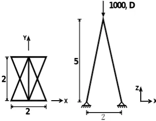
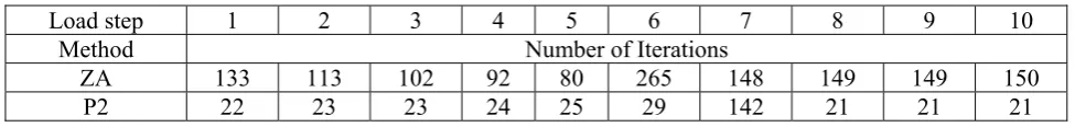
Figure 3 shows a three dimensional truss. The cross sectional area of members is 1 and the modulus of elasticity is 10 [3]. The load - displacement diagram has been drawn in Figure 4. In Table 2 the number of convergence iterations has been given.

8.3. Truss with 12 Members

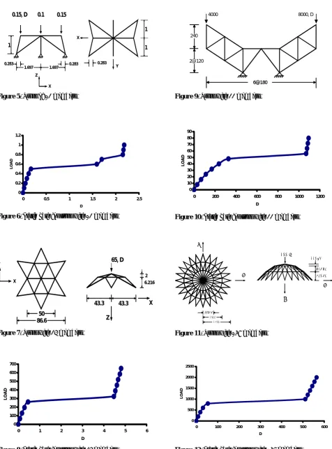
A three dimensional truss illustrating in Figure 5 has been examined. The area cross section of members is 1 and the modulus of elasticity is 10 [16]. The load - displacement diagram has been plotted in Figure 6. Table 3 shows the number of converged iterations for different schemes.

65.99 19.05

331600, D

Figure 1. Truss with two members.

0 500 1000 1500 2000 2500 3000 3500 4000 4500 5000

0 5 10 15 20

D

LOA

D

(9)

TABLE 1. Number of Iterations for Analysis of Two Member Truss.

10 9

8 7

6 5

4 3

2 1

Load step

Number of Iterations Method

152 152

152 153

153 153

154 162

ZA

21 21

P2

8.4. Truss with 24 Members

In order to assess the ability of new formulation efficiently, a larger system of equations should be solved. Now a truss with a larger degree of freedom is analyzed. This space truss has 24 members as shown in Figure 7. In this example, the member’s area cross sections are 3.17 cm2 _{and the modulus of elasticity} is 303000 N/cm2 _{[17]. The load - displacement} diagram and the number of iterations are shown in Figure 8 and Table 4, respectively.

8.5. Truss with 22 Members

A planer truss with 22 members is analyzed in constant load. This

truss is shown in Figure 9. In this example, the member’s area cross sections are 20 and 40 in2_for diagonal and other members, respectively. The modulus of elasticity is 30000 kips/in2_{[18]. The} load - displacement diagram is illustrated in Figure 10 and the number of converged iterations is listed in Table 5.

8.6. Truss with 168 Members

Figure 11 shows a truss with 168 members. Analysis of this example is performed under constant load. The area cross section of the members is 100 mm2_and the modulus of elasticity is 1000 N/mm2_{[19]. The} load - displacement diagram is illustrated in Figure 12. The number of iterations is given in Table 6.

9. CONCLUSIONS

In this paper, a new formulation for the DR method was suggested. Some planer and space trusses were also analyzed for numerical verification. The numerical results clarify that the new formulation increases the convergence rate as compare to the previous ones. As the applied mass in the suggested method is the one proportional to the stiffness matrix, different coefficients were investigated in this research. The results clearly establish that the coefficients less than 1 improve the convergence rate. By solving a variety of examples, this value was chosen 0.6 for all the structures.

On the other hand, not being able to trace the limitation points, like snap through in the static path, is the shortcoming of the new scheme as it is similar to the other DR methods. This characteristic is distinguishable in some examples such as example 2 that shows a big jump between the 6th and 7th step. This behavior raises the

2 2

Y

X

5

1000, D

Z

X

Figure 3. Truss with nine members.

0 2000 4000 6000 8000 10000 12000

0 2 4 6 8 10 12

D

LO

AD

(10)

TABLE 2. Number of Iterations for Analysis of Nine Member Truss.

10 9

8 7

6 5

4 3

2 1

Load step

150 149

149 148

265 80

92 102

113 133

ZA

21 21

21 142

29 25

24 23

23 22

P2

TABLE 3. Number of Iterations for Analysis of Truss with 12 Members.

10 9

8 7

6 5

4 3

2 1

Load step

28 29

91 219

129 20

22 29

36 50

ZA

11 11

95 171

155 13

12 11

11 11

P2

10 9

8 7

6 5

4 3

2 1

Load step

133 134

135 136

138 200

79 64

59 56

ZA

50 49

49 48

48 274

36 32

31 28

P2

TABLE 5. Number of Iterations for Analysis of Truss with 22 Members.

10 9

8 7

6 5

5 3

2 1

Load step

1286 1304

1142 3557

2436 1503

1052 783

633 577

ZA

1030 1054

993 3006

2285 1415

999 737

581 519

P2

10 9

8 7

6 5

4 3

2 1

Load step

768 774

780 787

795 1192

173 185

199 212

ZA

506 509

513 516

521 1016

119 116

150 171

P2

required number of iterations to find the next point on the static path.

Investigating the tables of converged iterations, a remarkable point is recognizable. There is an upsurge in the number of iterations by approaching the limit points of loads and displacements. In

(11)

0.283

1.697 0.283

0.15, D 0.1 0.15

Z

X

Y 1.697

1

0.283

1 1

Figure 5. Truss of 12 members.

0 0.2 0.4 0.6 0.8 1 1.2

0 0.5 1 1.5 2 2.5

D

LOAD

Figure 6. Static path for truss with 12 members.

50 86.6 X

Y

6.216 2 65, D

Z

X 43.3

43.3

Figure 7. Truss with 24 members.

0 100 200 300 400 500 600 700

0 1 2 3 4 5 6

D

LO

AD

6@180 6@180 2@120

240

4000 8000, D

0 10 20 30 40 50 60 70 80 90

0 200 400 600 800 1000 1200

D

LO

A

D

220.75

X

2900 1109.8 1109.8 2033

Z Y

200, D

940.83

X

628.64

0 500 1000 1500 2000 2500

0 100 200 300 400 500 600

D

LO

A

D

(12)

that contrary to the implicit scheme, there is no divergence when facing the limitation points.

10. NOTATION

[M] Mass matrix

[C] Damping matrix

[K] Stiffness matrix {x} Displacement vector

n

} x

{& Velocity vector in nth increment n

} x

{&& Acceleration vector in nth increment {Fi} Internal force of the ith degree of

freedom

{R}n Residual force

c Damp coefficient

e Allowable error

h Time increment

mij Diagonal entry of mass matrix n Number of step

KE Kinematic energy

α A real number

ωo The lowest natural period of the system

11. REFERENCES

1. Park, K. C., “A Famiy of Solution Algorithms for Non -

linear Structural Analysis Based on the Relaxation

Equations”, Int. J. Numer. Meth. Engng., 18, (1984),

1337-1347.

2. Zienkiewicz, O. C. and Lohner, R., “Accelerated

Relaxation or Direct Solution Future Prospects for

FEM”, Int. J. Num. Meth. Eng., Vol. 21, (1985), 1-11.

3. Rechardson, L. F., “The Approximate Arithmetical

Solution by Finite Difference of Physical Problems Involving Differential Equations, with an Application to the Stresses in a Masonary Dam”, R. Soc. London Phil. Trans. A 210, (1911), 307-357.

4. Casstell et al., “Cylindrical Shell Analysis by Dynamic

Relaxation”, Proc. Inst. Civ. Engrs., 39, (Jan. 1968),

75-84.

5. Welsh, A. K., “Discusstion on Dynamic Relaxation”,

Proc. Inst. Civ. Engrs., 37, (Aug. 1967), 723-750.

6. Rushton, K. R., “Large Deflection of Variable -

Thickness Plates”, Int. J. Mech. Sci., 10, (1968),

723-735.

7. Wood, W. L., “Comparison of Dynamic Relaxation

with Three Other Iterative Methods”, Engineer, 224,

(1967),683-687.

8. Felippa, C. A., “Dynamic Relaxation and Quasi-Newton

Method”, Numerical Pineridge Press, Sawnsea, UK, (1984).

9. Zhang, L. C., Kadkhodayan, M. and Mai, Y. W.,

“Development of the maDR Method”, Comput. Struc.,

Vol. 52, No. 1, (1994), 1-8.

10. Brew, J. S. and Brotton, M., “Non - Linear Sturctural

Analysis by Dynamic Ralaxation”, Int. J. Num. Meth.

Eng., Vol. 3, (1971), 463-483.

11. Underwood, P., “Dynamic Relaxation, in

Computational Method for Transient Analysis”, Chapter 5, Elsevier, Amesterdam, (1983), 245-256.

12. Zhang, L. C. and Yu, T. X., “Modified Adaptive

Dynamic Relaxation Method and Its Application to Elastic - Plastic Bending and Wrikling of Circular

Plates”, Comput. Struc., Vol. 34, No. 2, (1989),

609-614.

13. Shizhong, Q., “An Adaptive Dynamic Relaxation

Method for Non - Linear Problems”, Comput. Struc.,

Vol. 30, No. 4, (1988), 855-859.

14. Crisfield, M. A., “Nonlinear Finite Element Analysis of

Solids and Structures”, Advanced Topics, John Wiley and Sons Ltd., Vol. 2, (1997).

15. Ramesh, G. and Krishnamoorthy, C. S., “Inelastic Post -

Buckling Analysis of Truss Structures by Dynamic

Relaxation”, Int. Num. Meth. Eng., Vol. 37, (1994),

3633-3657.

16. Krenk, S. and Hededal, O., “A Dual Ortogonality

Procedure for Non - linear Finite Element Equations”,

Comput. Meth. Appl. Mech. Eng., Vol. 123, (1975),

95-107.

17. Ramesh, G. and Krishnamoorthy, C. S., “Post -

Buckling Analysis of Structures by Dynamic

Relaxation”, Int. Num. Meth. Eng., Vol. 36, (1993),

1339-1364.

18. Norris, C. H., Wilber, J. B. and Utku, S., “Elementary

Structural Analysis”, Third edition, McGraw Hill, NY, USA, (1976).

19. Forde, B. W. R. and Stiemer, S. F., “Improved Arc

Length Orthogonality Methods for Non - Linear Finite

Element Analysis”, Comput. Struc., Vol. 27, No. 5,