i
tif c n
e C
i o
c n
S f
l e
a r
n e
o n
i c
t e
a 2
nr 0
et 1
1
n I
ISC 2011
Proceeding of the International Conference on Advanced Science,
Engineering and Information Technology 2011
Hotel Equatorial Bangi-Putrajaya, Malaysia, 14 - 15 January 2011
ISBN 978-983-42366-4-9
ISC 2011
International Conference on Advanced Science, Engineering and Information Technology ICASEIT 2011
Cutting Edge Sciences for Future Sustainability
Hotel Equatorial Bangi-Putrajaya, Malaysia, 14 - 15 January 2011
SR
IE AUNVIIT NI
ESE
D K
O B
IN N
R AG
JA A
L S
A A
E N
P M
N A
A L
U A
T Y
A S
S A I
R
EP
N I
NOI TAI COSSA STNEDUTS NA IESODN Organized by Indonesian Students Association Universiti Kebangsaan Malaysia
Proceeding of the
Abstract— This paper presents a robust control design based on constrained optimization using Differential Evolution (DE). The
feedback controller is designed based on state space model of the plant considering structured uncertainty such that the closed-loop system would have maximum stability radius. A wedge region is assigned as a constraint for desired closed loop poles location. The proposed control technique is applied to a two-mass system that is known as benchmark problem for robust control design. The simulation results seem to be interesting in which the robustness performance is achieved in the presence of parameter variations of the plant.
Keywords— robust control, two-mass system, differential evolution
I. INTRODUCTION
Robustness has been an important issue in control systems design. A successfully designed control system should be always able to maintain stability and performance level in spite of uncertainties in system dynamics including parameter variations of the plant.
In robust control theory, H∞ optimization approach and the
µ-synthesis/analysis method are well developed and elegant [1]. They provide systematic design procedures of robust controllers for linear systems. However, the mathematics behind the theory is quite involved. It is not straightforward to formulate a practical design problem into H∞ or µ design
framework.
In this paper, we propose an alternative technique of robust feedback control design via constrained optimization. We employ DE (differential evolution) as a modern evolutionary algorithm that is fast and reasonably robust for optimization.
To deal with the plant’s parameter uncertainty, we employ complex stability radius as a tool of measuring system robustness. In addition, the desired response is automatically defined by assigning a regional closed loop poles placement. This region will be incorporated in the DE-based optimization as a constraint. In other word, the controller design technique is based on a constrained optimization to
obtain a set of feedback controller gains such that the closed-loop system would have maximum complex stability radius. At the end of this paper, we will present the simulation results of our proposed control design for two-mass system which is commonly known as a benchmark problem for robust control design [2-6].
II. BRIEF REVIEW
A. Problem Statement
Consider a plant model of linear time-invariant continuous-time system in state space form:
) ( ) ( )
(t Ax t But
x& = + (1)
) ( ) ( )
(t Cxt Dut
y = +
where x∈Rn , u∈Rm
and y∈Rp
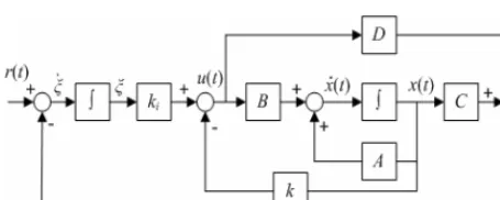
are state vector, control input and output vector respectively. It is assumed that the system given in (1) is completely state controllable and all state variables are available for feedback. One can use state feedback controller with feed-forward integral gain (ki) as shown in Fig. 1. The controller gains (k:=(k1,k2,k3,…kn)and ki) can be computed based on classical methods such as pole placement or linear quadratic optimal control via Riccati equation. These methods assume of course that there is no plant uncertainty.
Robust Control Design Based on Differential
Evolution for Two-Mass System
Mahmud Iwan Solihin# and Rini Akmeliawati*
#
School of Engineering, UCSI University
UCSI Heights, Cheras, 56000, Kuala Lumpur, Malaysia
*
Intelligent Mechatronics Systems Research Unit
Facultyof Engineering, International Islamic University Malaysia
Fig. 1. State feedback controller with feed-forward integral gain
In this work, constrained optimization using DE is employed to find a set of robust controller gains so that the plant uncertainty is automatically handled with the use of stability radius that will be discussed in the next section. In addition, a region of closed loop poles is incorporated as optimization constraint to allow the designers to define the desired control performance.
B. Stability radius
In this section, a tool of measuring system robustness is presented. It is called as stability radius [7]. It is a maximum distance to instability. Equivalently, a system having a larger stability radius implies that the system can tolerate more perturbations. In general, we can classify stability radius into two types; complex stability radius and real stability radius. Compared to real stability radius, complex stability radius can handle a wider class of perturbations including nonlinear, linear-time-varying, nonlinear-time-varying and nonlinear-time-varying-and-dynamics perturbations [8]. For this reason we use complex stability radius in this work. The complex stability radius will be maximized as in the optimization.
The definition of complex stability radius is given here. Let C denote the set of complex numbers. C-={z∈C|Real(z)<0} and C+=C\C- is the closed right half plane. Consider a nominal system in the form:
) ( )
(t Axt
x& = . (2)
A(t) is assumed to be stable. The perturbed open-loop system is assumed as:
) ( ) ) ( ) ( ( )
(t At E t H xt
x& = + ∆ (3)
where ∆(.) is a bounded time-varying linear perturbation. E and H are scale matrices that define the structure of the perturbations. The perturbation matrix itself is unknown. The stability radius of (3) is defined as the smallest norm of ∆ for which there exists a ∆ that destabilizes (2) for the given perturbation structure (E, H).
For the controlled perturbed system in the form (2), let:
E A sI H s
G 1
) ( )
( = − − (4)
be the “transfer matrix” associated with (A,E,H), then the complex stability radius is defined by the following definition.
Definition 1: [7] The complex stability radius, rc:
1
] ) ( [max ) , , ,
( −
∂ ∈ +
+
= Gs
C H E A r
C s c
, (5)
where ∂C+=C−∩C+ is the boundary of C+. In other words, a maximum rc can be achieved by minimizing the H∞ norm of the “transfer matrix” G [8].
III. DE-BASED CONTROL DESIGN
A. Brief Overview of DE
A DE algorithm is a stochastic search optimization method that is fast and reasonably robust. DE is capable of handling non-differentiable, non-linear, and multimodal objective functions [9]. DE is a one of the most promising novel evolutionary algorithms for solving global optimization problems [10]. It was proposed by Storn and Price not long ago in 1995 [11].
The structure of DE is similar to other evolutionary algorithms. The first generation is initialized randomly and further generations evolve by applying the evolutionary operators: mutation, recombination and selection to every population member until a stopping criterion is satisfied. There are some variants of DE. The DE variant called DE/rand/1/bin [12] is used here.
Furthermore, there are only few parameters defined by user in DE. Similar to other evolutionary algorithms, users have to select number of population, NP. The other control parameters are F (mutation scaling factor) and CR (crossover rate factor) which are normally valued between [0,1]. Users can refer to [13] for the choice of these parameters.
B. Constrained Optimization
The objective of the optimization is to maximize the complex stability radius (rc), however we will convert into minimization mode in this work by putting negative sign. Based on our approach, the searching procedure of the robust controller gains using constrained optimization can be formulated as follows (Table 1).
Table 1. Constrained optimization
Minimize: f(X)=−rc(X)
Subject to constraint: λn(X)∈ψ for n=1,2,…
and boundary constraint: X∈[lb,ub]
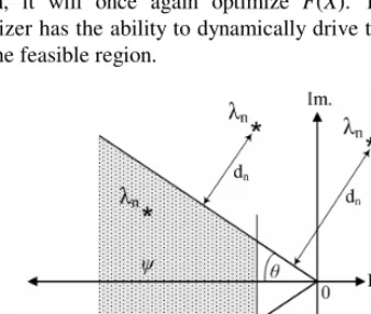
Fig. 2. A wedge region in complex plane for closed loop poles placement
X=K=(k1,k2,…,kn,ki) is the vector solutions such that
. 1 +
⊆
∈ n
R S
feasible region or the region of S for which the constraint is satisfied. The constraint here is the closed loop poles region; in the feasible region, the controller gains are found such that the closed loop poles (λ)lie within a wedge region (ψ ) of a complex plane as given in Fig. 2. The wedge region can be specified by two parameters θ and ρ which are related to desired transient response characteristics i.e.: damping ratio (ζ) and settling time.
C. Constraint Handling
An efficient and adequate constraint-handling technique is a key element in the design of stochastic algorithms to solve complex optimization problems. Although the use of penalty functions is the most common technique for constraint-handling, there are a lot of different approaches for dealing with constraints [14].
Instead of using penalty approach like in [15] where the optimizer seemed to be inefficient (high iterations), we adopt a dynamic-objective constraint-handling method (DOCHM) [16] in order to improve the efficiency. Through defining distance function F(X), DOHCM converts the original problem into bi-objective optimization problem min(F(X),f(X)), where F(X) is treated as the first objective function and f(x) is the second (main) one.
The auxiliary distance function F(X) will be merely used to determine whether or not an individual (candidate of solution) is within the feasible region and how close a particle is to the feasible region. If an individual lies outside the feasible region (at least an eigenvalue lies outside the wedge region), the individual will take F(X) as its optimization objective. Otherwise, the individual will instead optimize the real objective function f(X). During the optimization process if an individual leaves the feasible region, it will once again optimize F(X). Therefore, the optimizer has the ability to dynamically drive the individuals into the feasible region.
Fig. 3. Eigenvalue distance to the wedge region in complex plane
The procedure of the DOCHM applied to the eigenvalue assignment in the wedge region is illustrated in the following pseudo-code (Table 2). Referring to Fig. 3, let dn is an outer distance of an eigenvalue (λn) to the wedge region. It is noted that if an eigenvalue lies within the wedge region, dn=0. F(X) is defined by:
∑
+= =
1
1
))) ( ( , 0 max( )
(
n
i
n
n X
d X
F λ (6)
Table 2. Pseudo-code for constraint handling
If F(X)=0
) ( )
(X r X
f =−c
Else
) ( )
(X F X
f =
End
D. Stopping criterion
In literatures, mostly two stopping criteria are applied in single-objective optimization: either an error measure if the optimum value is known is used or the number of function evaluations (number of iterations). There are some drawbacks for both. The optimum has to be known in the first method, so it is generally not applicable to real-world problems because the optimum is usually not known a priori. The second method is highly dependent on the objective function. Because generally no correlation can be seen between an optimization problem and the required number of function evaluations (iterations), it has to be determined by trial-and-error methods usually. Improper selection of the number of iterations to terminate the optimization can lead to either premature convergence or expensive optimization runs (excessive computational effort).
As a result, it would be better to use stopping criterion that consider knowledge from the state of the optimization run. The time of termination would be determined adaptively, so the optimization run would be efficient. Several stopping criterions are reviewed in [17]. Although the authors did not conclude which one is the best for all problems, it is believed that performance improvement can be obtained with adaptive stopping criterion.
In this work, we adopt the stopping criterion which is distribution-based criterion which considers the diversity in the population. If the diversity is low, the individuals are close to each other, so it is assumed that convergence has been obtained [17]. Standard deviation (σ) of the best individuals in each dimension during iterations is checked. If it is below a threshold
ε
(small number) for sufficiently large number of iterationsη
, the optimization will be terminated. It can be formulated as in Table 3; wherej d best
x , represents the best individual in j-th generation
(iteration) for d dimension.
Table 3. Stopping criterion If
)) min( ) (max( )
( 1
, ,
1
2 ,
, bestd bestd
j
d best j
d best
d =
∑
x −x < x − x=
ε η
σ
η
(for d=1,2,…,D)
stop iterations.
End
IV. ROBUST CONTROL DESIGN FOR TWO-MASS SYSTEM
[5]. Consider the two-mass system shown in the Fig. 4. A control force (u) acts on body 1 and the position of body 2 is measured. Both masses are equal to one unit (m1=m2=1) and the spring constant is assumed to be in the range 0.5≤k≤2. The system can be represented in state space form:
u x x x x k k k k x x x x + − = 1 0 0 0 0 0 0 0 1 0 0 0 0 1 0 0 4 3 2 1 4 3 2 1 & & & & (12)
where: x1: position of mass-1 x2: position of mass-2 x3: velocity of mass-1 x4: velocity of mass-2
Fig. 4. Two-mass and spring system
The plant uncertainty is due to variations of the spring constant where the nominal value is selected for the worst case of k=0.5. Therefore uncertainties appear in the rows 3-4 and the columns 1-2 of the state matrix. The scale matrices as the perturbation structure for the closed loop system are Ecl and Hcl whose diagonal elements in rows 3-4 of Ecl and in columns 2-3 of Hcl are respectively equal to 1.
= 0 0 0 0 0 0 1 0 0 0 0 0 1 0 0 0 0 0 0 0 0 0 0 0 0 cl E = 0 0 0 0 0 0 0 0 0 0 0 0 0 0 0 0 0 0 1 0 0 0 0 0 1 cl H
The next is to choose the parameters of the wedge region (Fig. 2) whose role is to locate the closed loop poles. The damping ratio is usually set to ζ=0.7 to produce sufficient overshoot damping in the response. The transient margin (ρ) is specified according to the desired speed of the response. This is problem-dependent parameter. Here, we set ρ=1. In addition, the main DE-based optimization parameters are listed in Table 4.
Table 4. DE-based optimization parameters
Dimension of the problem D 5
Population size NP 100
Mutation scaling constant F 0.9
Crossover rate constant CR 0.5
Upper and lower bounds of solution ±BD ±50
Maximum iteration jmax 2000
Number of iteration for which stopping criterion
applies η 200
Standard deviation threshold for which
stopping criterion applies ε 1%
V. RESULTS
The optimization run has been performed in MATLAB 2006. Since DE is a stochastic optimization, a number of optimization runs need to be executed with different initial random seeds. To get an optimal solution and to evaluate the quality of the solution (robustness, convergence, repeatability), 15 runs have been executed here. The mean value, the standard deviation of the fitness value (f(X)=-rc) and other results are recorded in Table 5.
Table 5. Optimization results for 15 runs
Average f(X) -0.32
Median f(X) -3.07
Standard deviation f(X) 0.005
Range of f(X) -0.31 to -0.33
Average number of iteration 715
Average computation time 0.77 minutes
Table 6. Controller gains for two-mass system
k1 k2 k3 k4 ki
Controller
gains 18.49 19.04 47.27 7.30 -10.54
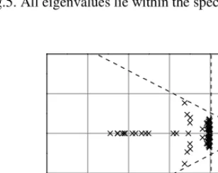
Form Table 5, it can be seen that the optimization results in a robust solution with a small standard deviation, the range of the fitness value is also very small. This means that the optimizer has a good repeatability property. The distribution of eigenvalues for those 15 runs can be seen in Fig.5. All eigenvalues lie within the specified wedge region.
-5 -4 -3 -2 -1 0-4
-2 0 2 4 I m a g in a ry Real
Fig. 5. . Distribution of eigenvalues within the wedge region for 15 runs
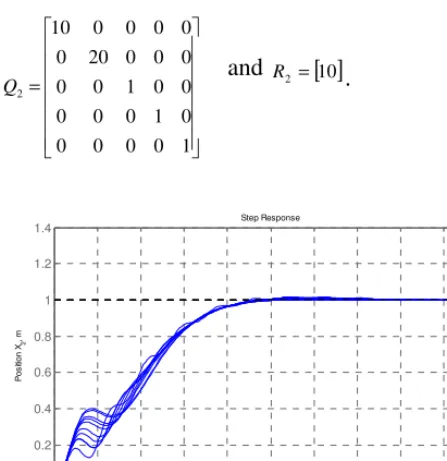
Furthermore, to see the controller performance, a set of controller gains is picked from the median data and it is shown in Table 6. Fig. 6 shows 10 random samples (with 10 random values of the spring constant 0.5≤k≤2) of step response (position of mass-2) with the proposed DE-based feedback controller (DEFC). For comparison, two conventional LQR-based controllers (linear quadratic regulator) are also designed with the following sets of Q and R matrices respectively for LQR1 and LQR2:
= 100 0 0 0 0 0 1 0 0 0 0 0 1 0 0 0 0 0 1 0 0 0 0 0 10 1
=
1 0 0 0 0
0 1 0 0 0
0 0 1 0 0
0 0 0 20 0
0 0 0 0 10
2
Q
and
R2 =[ ]
10.
0 2 4 6 8 10 12 14 16 18 20
0 0.2 0.4 0.6 0.8 1 1.2
1.4 Step Response
Time, s (sec)
P
o
s
iti
o
n
X2
,
m
Fig. 6. Ten random samples of step response for DEFC
Figs. 7-8 show 10 random samples of the step response (the position of mass-2) for LQR1 and LQR2 respectively. It can be seen that the proposed controller (DEFC) is more robust compared to the two LQR-based controller (LQR1 and LQR2) designed in this work.
0 2 4 6 8 10 12 14 16 18 20
0 0.2 0.4 0.6 0.8 1 1.2 1.4
Step Response
Time (sec)
P
o
s
iti
o
n
X2
,
m
Fig. 7. Ten random samples of step response for LQR1
0 2 4 6 8 10 12 14 16 18 20
0 0.1 0.2 0.3 0.4 0.5 0.6 0.7 0.8 0.9
1 Step Response
Time (sec)
P
o
s
iti
o
n
X2
,
m
Fig. 7. Ten random samples of step response for LQR2
VI. CONCLUSIONS AND DISCUSSIONS
A robust state feedback control design via constrained optimization using DE has been presented. The designed controller has shown a robust performance in the presence of parameter variations. The DE-based constrained optimization effectively locates closed loop poles within a prescribed wedge region and able to maximize the stability radius with a good repeatability of the solution.
Finally, this paper reports a preliminary research. To further evaluate the robust performance of the proposed controller, it is necessary to analyze in more detail using robust control concepts. Comparison with other robust control techniques is also necessary. This will be done in the future.
REFERENCES
[1]. Gu, D.W., Petkov, P.H., Konstantinov, M.M. (2005). Robust Control Design with MATLAB. Springer-Verlag, London. [2]. Ly, U.L. (1990). Robust control design using nonlinear constrained
optimization. Benchmark problems for robust control design. Procs. of American Control Conference, pp. 968-969.
[3]. Rotstein, H and Sideris, A. (1991). Constrained H∞ optimization: A design example. Procs. of the 30th Conference on Decision and Control.
[4]. Byrns, E.V and Calise, A.J. (1992). A loop transfer recovery approach to H∞ design for the coupled mass benchmark problem. Journal of Guidance, Control, and Dynamics. Vol. 15, no. 5, pp. 1118-1124
[5]. Wie, B and Berstein, D.S. (1990). Benchmark problems for robust control design. Procs. of American Control Conference, pp. 961-962. [6]. Petersen, I.R., Ugrinovskii, V.A and Savkin, A.V. (2000). Robust
control design using H∞ method. Springer-Verlag. pp.151-155. [7]. Hinrichsen, D and Pritchard, A.J. (1986). Stability radii of linear
systems. Systems & Control Letters, 7:1–10.
[8]. Akmeliawati, R., and Tan, C. P. (2005). Feedback controller and observer design to maximize stability radius. Proceedings of the International Conference on Industrial Technology, pp. 660-664. [9]. Weisstein E.W., Vassilis P. (2006). Differential evolution. Web
resource; http://mathworld.wolfram.com/DifferentialEvolution.html. [10]. Yousefi, H., Handroos, H., Soleymani, A. (2008). Application of
differential evolution in system identification of a servo-hydraulic system with a flexible load, Mechatronics 18 : 513–528
[11]. R. Storn and K. Price. (1995). Differential evolution-a simple and efficient adaptive scheme for global optimization over continuous spaces. Technical Report, International Computer Science Institute. [12]. K. V. Price. (1999). An introduction to differential evolution, in New
Ideas in Optimization, D. Corne, M. Dorigo, and F. Glover, Eds. London: McGraw-Hill, pp. 79–108.
[13]. R. Storn. (1996). On the usage of differential evolution for function optimization. In IEEE Biennial Conference of the North American Fuzzy Information Processing Society, pp. 519-523.
[14]. Coello Coello, C.A. (2002). Theoretical and numerical constraint-handling techniques used with evolutionary algorithms: A survey of the state of the art. Computer Methods in Applied Mechanics and Engineering, vol. 191, no. 11-12, pp. 1245–1287.
[15]. Solihin, M.I, Wahyudi, Legowo, A and Akmeliawati, R. (2009). Self-erecting inverted pendulum employing PSO for stabilizing and tracking controller. Procs. of 5th International Colloquium on Signal Processing & Its Applications, pp.63-68.
[16]. Lu, H. and Chen, W. (2006). Dynamic-objective particle swarm optimization for constrained optimization problems. Journal of Global Optimization, 12:409-419.