R E S E A R C H
Open Access
Modelling stochastic correlation
Long Teng
*, Matthias Ehrhardt and Michael Günther
*Correspondence:
[email protected] Lehrstuhl für Angewandte Mathematik und Numerische Analysis, Fakultät für Mathematik und Naturwissenschaften, Bergische Universität Wuppertal, Gaußstraße 20, Wuppertal, 42119, Germany
Abstract
This work deals with the stochastic modelling of correlation in finance. It is well known that the correlation between financial products, financial institutions, e.g., plays an essential role in pricing and evaluation of financial derivatives. Using simply a constant or deterministic correlation may lead to correlation risk, since market observations give evidence that the correlation is hardly a deterministic quantity. For example, we illustrate this issue with the analysis of correlation between daily returns time series of S&P Index and Euro/USD exchange rates.
The approach of modelling the correlation as a hyperbolic function of a stochastic process has been recently proposed. Here, we review this novel concept and generalize this approach to derive stochastic correlation processes (SCP) from a hyperbolic transformation of the modified Ornstein-Uhlenbeck process. We determine a transition density function of this SCP in closed form which could be used easily to calibrate SCP models to historical data.
As an illustrating example of our new approach, we compute the price of a quantity adjusting option (Quanto) and discuss concisely the effect of considering stochastic correlation on pricing the Quanto.
Keywords: stochastic correlation; quanto option; correlation risk;
Ornstein-Uhlenbeck process; transition density; hyperbolic tangent function
1 Introduction
Correlation is a well established concept for quantifying the relationship between financial assets. It plays an essential role in several financial applications, e.g. the arbitrage pricing model [] is based on correlation as a measure for the dependence of assets. Also in port-folio credit models, the default correlation is one fundamental factor of risk evaluation, see e.g. [] and [].
For two random variables X andX with finitevariances, thecorrelationof them is
defined as
ρ,=Corr(X,X) =
Cov(X,X) σσ
, ()
with thecovariance
Cov(X,X) =E
(X–μ)(X–μ)
, ()
whereμiandσiare theexpectationandstandard deviationofXi,i= , . Hereρ,denotes
a coefficient number in the interval [–, ]. The boundaries – and will be reached if and
only ifX andX are indeed linearly related. The greater the absolute value ofρ,the
stronger the dependence betweenXandXis.
Generally, there are several disadvantages or fallacies of the correlation concept (), we state only some of them:
• If the random variablesXandXare independent, then it followsρ,= . However,
the converse implication does not hold, since in () only the two first moments are included. For example, we computeρ,= forX=X. Indeed,XandXdepend
even almost perfectly on each other. This illustrates that the correlation coefficient only recognizes linear dependencies between random variables.
• Correlation is invariant under strictly increasing linear transformations, but, in contrast to Copula methods, not invariant under nonlinear strictly increasing transformations. For example, in general the correlation of the random variablesX
andXdoes not equal the correlation of the random variableslnXandlnX, i.e. after a transformation of the financial data the correlation may change.
• Usually, the given marginal distributions and pairwise correlations of a random vector cannot determine its joint distribution.
• Finally, as stated above, the variances of the two random variablesXandXhas to be finite. This assumptions is not fulfilled for every standard distribution, e.g. the Student’st-distribution withv≤possess an infinite variance.
For more detailed information about the disadvantages or fallacies we refer to []. Al-though this concept of correlation () to measure dependence inherits several limitations, it has been widely applied in financial applications.
In financial markets, the first problem of using a correlation concept is theobservability. Unlike prices, volatilities, exchange rates and so on, the correlation cannot be observed directly in the market and can only be measured in the context of a model. The easiest estimator of the correlation is the sample correlation coefficient. Given a series ofN mea-surements ofXandX, which are observable quantities in the market, and denoting the measurements byx,jandx,j,j= , , . . . ,N, thesample coefficient correlationreads
ˆ
ρ=
N
j=(x,j–μ¯)(x,j–μ¯)
N
j=(x,j–μ¯)
N
j=(x,j–μ¯)
, ()
whereμ¯andμ¯are thesample meansofXandX.
In financial models, stochastic processes are used quite often to model data series, like price, interest rate and exchange rate. When considering diffusion processes, the depen-dence between the series is given bycorrelated Brownian motions. Two Brownian motions
WandWare correlated by the symbolic notion
dW,tdW,t=ρ,dt. ()
For example, in the multivariate Black-Scholes model, the correlation of the log-returns is used as a measure of the dependence between asset processes. A further example of
coupled stochastic processes appears when pricing aquantity adjusting option (Quanto)
in the framework of the Black-Scholes model: ⎧
⎨ ⎩
dSt=μSStdt+σSStdWtS,
dRt=μRRtdt+σRRtdWtR,
with positive constantsμS,μR,σSandσR. The firststochastic differential equation (SDE) describes the price, St of the traded asset in a currency A. The second SDE is used to
model the exchange rate Rt between currency A and another currency B. Besides, the
Brownian motions are assumed to be correlated by a constant correlationρ∈[–, ] which is a measure of co-movements betweenStandRt.
As we explained above, the constant correlation coefficient defined by () only captures linear relationships betweenXandX. Therefore, in the model () a linear dependence betweenSt andRt is assumed. However, from the market we realize that there is often a nonlinear dependence betweenSt andRt. Specifically, a constant correlation means that the two return processes are jointly stationary which is generally not true in the real world. Thus, the dependence can be hardly modelled by a fixed constant, i.e. the constant cor-relation may not be an appropriate measure of co-dependence. Using constant (“wrong”) correlation may result some ’correlation risk’. There exist already some works which show that the correlation should not be constant and even changes over a small time interval as the volatility, see e.g. []. Several approaches generalize the constant correlation to a time-varying and stochastic concept, likeDynamic Conditional Correlation modelin [],
Local correlation modelssee e.g. [] and theWishart autoregressive processproposed by Gourieroux [] that guarantees the positive definiteness of the variance-covariance ma-trix.
In fact, either implied correlation in the context of a model or historical correlation from the market data show us that the correlation should be time-varying and behave like a stochastic process. To illustrate this statement, we make an example of historical correla-tions betweenS&P indexandEuro/US-Dollar exchange rateon a daily basis. We use ¯
sandr¯to denote the daily return series of S&P and Euro/US-Dollar exchange rate and fix a time windownT, e.g.nT= for -day historical correlation. At timet, using thenTtimes most recent daily returns, the correlation at timetis given by the following estimator
ˆ
ρt=
nT
j=(ˆst–j–nT nT
j=ˆst–j)(ˆrt–j–nT nT
j=rˆt–j)
nT
j=(sˆt–j–nT nT
j=ˆst–j) nT
j=(ˆrt–j–nT nT
j=ˆrt–j)
. ()
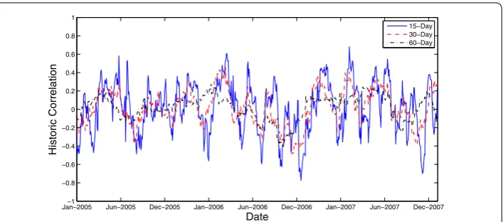
Then we roll it to the timet+ , and so on to obtain a series of correlations through the time. The -day, -day and -day historical correlations are displayed in Figure .
We observe that the longer a time window (the value ofnT) the less volatile a historical correlation is. In Figure , the -day historical correlation is more variable than the -day historical correlation which is again more variable than the --day correlation. With a longer averaging period along-term correlationis calculated. If we choosenT= or days, the estimated correlation for each time tusing (), could be seen as ashort-term correlationof the current market phenomena whose immediate past returns are used for the estimation. It is worthwhile noting that the events, especially, some extreme events in a time window will affect the correlation which would be estimated in the following time windows, even has a delayed effect on the long-term correlation.
Figure 1 Historical correlation between S&P 500 and Euro/US-Dollar exchange rate, source of data: www.yahoo.co.
Figure 2 Empirical density function of the historical correlation between S&P 500 and Euro/US-Dollar exchange rate.
the variation of the short-term correlation can be reflected, also the attributes of long-term correlation is determined by the long-term parameter values, like long-term mean value and mean reversion speed.
To see more properties, which a mean-reverting stochastic process should have to be a SCP, we plot its empirical density functions in Figure using different bandwidths. We refer to [] for details about the estimation of a density function from historical data.
From studying the empirical density functions we require that thestochastic correlation processshould satisfy the following properties:
(i) only takes values in the interval(–, ), (ii) varies around a mean value,
(iii) the probability mass tends to zero at the boundaries–,+.
hyper-bolic tangentfunction of any mean-reverting process with positive and negative values, the properties (i)-(iii) above can be thus directly satisfied without facing any additional parameter restrictions. Hence, the subsequent calibration process is much simpler.
In this work, we study the general SCP by Teng et al. []. We show that the correla-tion process by van Emmerich can be obtained by this general method, i.e. the correlacorrela-tion process by van Emmerich turns out to be a special case of the hyperbolic transformation of a stochastic process. Furthermore, we apply this general approach to find a new SCP which has a transition density function in closed form. Finally, as an illustrating exam-ple, we compute the price of a Quanto under stochastic correlation by our new SCP and investigate the effect of considering stochastic correlation on pricing the Quanto.
2 A general stochastic correlation model
Here we study the hyperbolic transformation proposed in [] of a mean-reverting process to be a correlation process. We show that the correlation process model of van Emmerich [] can be obtained by transforming a mean-reverting process with the hyperbolic tan-gent function. We fix a probability space (,F,P) and an information filtration (Ft)t∈R+ satisfying the usual conditions, see e.g. [].
2.1 The transformed mean-reverting process
For the motivations and the properties (i)-(iii) in Section , Teng et al. [] proposed the hyperbolic tangent function of a mean-reverting stochastic processXt, like the Ornstein-Uhlenbeck process [] or the square root diffusion processes (with positive and negative values)
dXt=a(t,Xt)dt+b(t,Xt)dWt, t≥,X=x, ()
to model the correlations as
ρt=tanh(Xt), ρ=tanh(x)∈(–, ). ()
Obviously, the properties (i)-(iii) are fulfilled due to the range of values of the hyperbolic tangent function and mean reversion of the process. Besides, the function tanh is sym-metrical and measurable. Although the function tanh can not really attain – and which presents perfect negative and perfect positive dependence, respectively. It should make no difference to use this function for modelling correlations, because the correlation equal to – or is indeed an extreme event which happens very rarely in the real market, see e.g. Figure . Besides, the function tanh tends to the boundaries – and at infinity.
ApplyingItô’s Lemmawith ()
dρt=dtanh(Xt) =
∂tanh(Xt)
∂t dt+
∂tanh(Xt)
∂x dXt+
∂tanh(Xt)
∂x (dXt)
, ()
we obtain thestochastic correlation process (SCP)
dρt= –ρt
˜
a–ρtb˜
dt+b dW˜ t
, t≥, ()
is obvious that, in this approach any mean-reverting process (with positive and negative values) can be considered without facing any additional parameter restrictions. The free parameters are hidden in the functionsaandb, see the example () in Section . and () in Section ..
2.2 Transformation with other functions
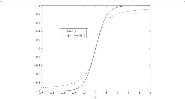
Although we could intuitively observe that the functiontanh(x) is eminently suitable for correlation modelling, one can still ask whether other functions having values inside the interval (–, ), like trigonometric functions or πarctan(πx),x∈Rcan also be applied for this purpose? In theory, such functions could be used for the SCP model above. However, the trigonometric function is a periodic function, the arising complex number will com-plicate further calculations. For the functionπarctan(πx), its Itô’s formula for () is given by
dρt=d
πarctan
π
Xt
=
˜
a
( +tan(ρtπ
))
– πb˜
tan(ρtπ )
( +tan(ρtπ
))
dt
+ b˜
( +tan(ρtπ ))
dWt, ()
which is rather complicate such that the further computation will be tedious.
Further-more, we compare the function
πarctan( π
x) withtanh(x) in Figure and find that the
both function are close to each other in the neighbourhood ofx= . However, compared
withtanh(x), the functionπarctan(πx) grows much slower up to and down to –, so that the estimation of the correlation will be worsened. The reason is similar to the estimation for the heavy tailed distributions.
2.3 The correlation model of van Emmerich
As an example, we show that the correlation model of van Emmerich can be obtained by transforming the special mean-reverting process (), i.e. the van Emmerich’s correlation
process is just a special case of the general transformation []. To do so, we define the following mean-reverting process
dXt=
κ(μ–tanh(Xt)) –tanh(Xt)
dt+ σ –tanh(Xt)
dWt, t≥,X=x, ()
whereκandσ are positive,μ∈(–, ). Next, we transform () withρt=tanh(Xt). Again, applying Itô’s Lemma we obtain after a tedious calculation
dρt= κ(μ–ρt)
–σρt
dt+σ
–ρ
t dWt. ()
Next, if we define
κ∗=κ+σ, μ∗= κμ
κ+σ, σ
∗=σ ()
the correlation process () can be rewritten as
dρt=κ∗ μ∗–ρt
dt+σ∗
–ρtdWt, ()
which is exactly the van Emmerich’s correlation process in []. Due to the transformation with the function tanh, the correlations provided by (), with coefficients (), are obvi-ously located in the interval (–, ). We can check this important property in another way: We recall that van Emmerich [] derived the analytic condition
κ∗≥ σ
∗
±μ∗ ()
to ensure that the boundaries – and are unattainable. We see that the correlation process () must have already satisfied the condition (): Substituting () in () we obtain
σ
κ(±μ) +σ ≤, ()
which always holds whilstκis positive andμ∈(–, ).
3 Stochastic correlation with a modified Ornstein-Uhlenbeck process
In this section, we specify a SCP by a hyperbolic transformation of the modified Ornstein-Uhlenbeck process. The derivation of the transition density function of this SCP is pro-vided in a closed form. Then, we analyse this density function and show how to fit the correlation process to the historical market data.
3.1 The transformed modified Ornstein-Uhlenbeck process TheOrnstein-Uhlenbeck processis defined by the SDE
dXt=κ(μ–Xt)dt+σdWt, ()
whereκ,σ> andX,μ∈R. If we want to restrict the mean reversion valueμto be only in (–, ), it is reasonable to modify the Ornstein-Uhlenbeck process () as
dXt=κ μ–tanh(Xt)
whereκ,σ> andX,μ∈(–, ).
Lemma The SCPρt=tanh(Xt)satisfies the SDE
dρt= –ρt κ(μ–ρt) –σρt
dt+ –ρtσdWt, ()
where t≥,ρ∈(–, ),κ,σ> andμ∈(–, ).
Proof Applying Itô’s Lemma we obtain
dρt=
∂tanh(Xt)
∂x dXt+
∂tanh(Xt)
∂x σ dt
=sech(Xt)κ μ–tanh(Xt)
dt–sech(Xt)
sinh(Xt)
cosh(Xt)
σdt+sech(Xt)σdWt
= –ρtκ(μ–ρt)dt– –ρt
ρtσdt+ –ρt
σdWt= ().
Let us introduce the notation
κ∗=κ+σ, μ∗= κμ
κ+σ, σ
∗=σ. ()
and rewrite () as
dρt –ρ
t
=κ∗ μ∗–ρt
dt+σ∗dWt, ()
wheret≥,ρ∈(–, ),κ∗,σ∗> andμ∗∈(–, ).
3.2 Transition density function
For calibration purposes, we first determine thetransition density functionof () with the aid of theFokker-Planck equation[]. Then, we obtain the parameters of the correlation process () by fitting the density function to the market data.
Let us assume that the SCP () possesses a transition densityf(t,ρ˜|ρ) which satisfies
the following Fokker-Planck equation
∂
∂tf(t,ρ˜) + ∂
∂ρ˜ aˆ(t,ρ˜)f(t,ρ˜)
–
∂ ∂ρ˜ bˆ(t,ρ˜)
f(t,ρ˜)= , ()
with
ˆ
a(t,ρ˜) =κ∗ μ∗–ρ˜ –ρ˜, bˆ(t,ρ˜) = –ρ˜σ∗. ()
For the calibration purpose we consider the stationary density (fort→ ∞)
f(ρ˜) :=lim
t→∞f(t,ρ˜|ρ). ()
In the sequel, we show how to determine the analytical stationary density functionf(ρ˜) of the SCP (). First, the stationary density functionf(ρ˜) obviously satisfies
∂ ∂ρ˜
–ρ˜ κ∗ μ∗–ρ˜f(ρ˜)=
∂ ∂ρ˜
–ρ˜σ∗f(ρ˜). ()
By solving the elliptic equation () with the aid of using Maple we obtain the stationary densityf(ρ˜) as
f(ρ˜) = m κ
∗
σ∗ ( +ρ˜)
κ∗–σ∗ σ∗ +
κ∗μ∗ σ∗ ( –ρ˜)
κ∗–σ∗ σ∗ –
κ∗μ∗ σ∗
+ n
˜
ρ–
σ∗–κ∗ σ∗
F
,σ
∗– κ∗
σ∗ ,
(–μ∗– )κ∗+ σ∗
σ∗ ,
˜ ρ + ()
with the constantsm,n∈Rand thehypergeometric function Fwhich is defined as
F(a,b,c,x) =
∞
k= xk
k!
(a)k(b)k (c)k
, |x|< , ()
where (·)kdenotes thePochhammer symbol,
(a)k=a(a+ )(a+ )· · ·(a+k– ), (a)= . ()
Next we need to fix the constantsmandnin () to obtain the stationary density. Due to the mean reversion the stationary densityf(ρ˜) must satisfy
–
˜
ρf(ρ˜)dρ˜=μ∗.
If we chooseμ∗= , we observe that the first term in () becomes
m
κ
∗
σ∗
( +ρ˜)κ
∗–σ∗
σ∗ ( –ρ˜) κ∗–σ∗
σ∗ , ()
which is obviously symmetric aroundρ˜= , i.e. the condition () will be fulfilled forn= . In the sequel we assume thatn≡ for all generalμ∗∈(–, ) such that the transition density function () can be rewritten as
f(ρ˜) = m κ
∗
σ∗
( +ρ˜)κ
∗–σ∗
σ∗ + κ∗μ∗
σ∗ ( –ρ˜) κ∗–σ∗
σ∗ – κ∗μ∗
σ∗ . ()
To determine the value ofmwe can employ the basic property of a density function
–
f(ρ˜)dρ˜= . ()
The constantmin () must be chosen such that the normalization condition () is always fulfilled. We set
a=κ
∗– σ∗
σ∗ , b= κ∗μ∗
and substitute it into () to obtain
f(ρ˜) = m κ
∗
σ∗
( +ρ˜)a+b( –ρ˜)a–b. ()
As long as
a±b> –, ()
the integral
–
( +ρ˜)a+b( –ρ˜)a–bdρ˜
has the solution
M:=( +a–b)F(, –a–b, +a–b, –)
( +a–b)
+( +a+b)F(, –a+b, +a+b, –)
( +a+b) , ()
with the hypergeometric functionFdefined in () and thegamma function.
Next we show that ifμ∈(–, ) then () holds. Using the definitions ofκ∗,μ∗andσ∗
in () and together with () we obtain
a=κ
∗– σ∗ σ∗ =
κ–σ
σ , b= κ∗μ∗
σ∗ = κμ
σ. ()
We consider the following simple calculations
μ> –⇒κ( +μ) > ⇒κ–σ
σ + κμ
σ > –⇒a+b> –,
μ< ⇒κ( –μ) > ⇒κ–σ
σ – κμ
σ > –⇒a–b> –
and realize that the condition () will always hold due toμ∈(–, ). Thus, the constant
mcan be determined as
m= κ∗ σ∗
M . ()
Finally, we obtain the transition density function in a closed form as
f(ρ˜) =( +ρ˜)
a+b( –ρ˜)a–b
M , ()
witha,bdefined in () andMin (). The parametersκ∗,μ∗andσ∗, or rather,κ,μand
We could generalize the correlation process () with the same definition but directly with the arbitrary parameter coefficientsκ> ,μ∈(–, ) andσ> , like
dρt
–ρt =κ(μ–ρt)dt+σdWt. ()
For this case, we have foraandb, as defined in (), as
a=κ– σ
σ , b=
κμ
σ. ()
We perform a similar calculation for checking the condition () as above:
a+b> –⇐κ– σ
σ + κμ
σ > –⇐κ( +μ) >σ
⇐κ> σ
+μ,
a–b> –⇐κ– σ
σ – κμ
σ > –⇐κ( –μ) >σ
⇐κ> σ
–μ.
Thus, the process () could be employed for the stochastic correlation if the condition
κ> σ
±μ ()
is fulfilled. We find that this condition dovetails nicely with that condition in [], which ensures that the boundaries – and are unattainable.
To further illustrate the transition density functionf(ρ˜), we display in Figures , and the behaviour off(ρ˜) for different values of each parameter. In Figure , we letκ= and
μ= and displayf(ρ˜)ith different values ofσ, which is equal to ., . and ., respec-tively. Obviously,σshows the magnitude of variation from the mean valueμ= . Next, we fixκ= andσ= ., the behaviour off(ρ˜) only with varying mean valueμ= –.,μ= andμ= . can be found in Figure . However, whilstμ= –. andμ= . we can observe that the peak of the correspondingf(ρ˜) does not locate exactly at the pointsρ˜= –. and
˜
ρ= ., respectively. The reason is that, the value ofκ, which is mean reversion rate, is not large enough. In order to illustrate the role ofκ, we setμ= –.,σ= . and vary the value
Figure 5 Comparison off(ρ˜) for different values ofμ(κ= 2 andσ= 0.3).
Figure 6 Comparison off(ρ˜) for different values ofκ(μ= –0.5 andσ= 0.5).
ofκ, see Figure . Forκ= , the peak of the transition density function is far away from the mean value –.. However, in contrast the peak reaches already the pointρ˜= –. when
κ= .
3.3 Calibration
We assume that the correlation is itself observable. Under this assumption the transition density can be used for calibration purposes. One uses usuallymaximum-likelihood esti-mation (MLE)when the density function is known. Considering the density function (), it will be tedious to determine its likelihood-function.
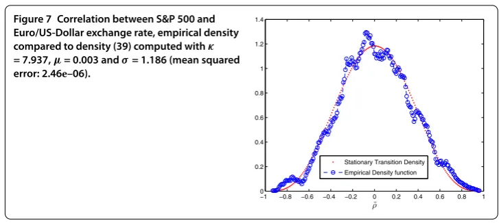
Another approach to estimate the parameters is to fit the empirically observed density to the stationary density (). As an example we fit the historical data from Figures a to (). The fitting by nonlinear least-squares works well, see Figure .
4 Stochastically correlated Brownian motions
Figure 7 Correlation between S&P 500 and Euro/US-Dollar exchange rate, empirical density compared to density (39) computed withκ
= 7.937,μ= 0.003 andσ= 1.186 (mean squared error: 2.46e–06).
need the concept ofstochastically correlated Brownian motions. In the following, we study the stochastically correlated Brownian motions following the work of van Emmerich [].
Based on two independent Brownian motionsW,tandW,twe define
W,t= t
ρsdW,s+ t
–ρ
sdW,s, ()
whereρt is one SCP of type (), and we assume thatWt in () is independent of each
Wi,t, fori= , .
Lemma W,tsatisfies () W,= ,
() E[(W,t)] =t,
() E[W,t|Fs] =W,s,fors≤t.
Proof () is obvious. We calculate the two expected values as follows:
E(W,t)
=E
t
ρsdW,s
+
t
–ρ
sdW,s
+ t
ρsdW,s t
–ρ
sdW,s
=E
t
ρsds+
t
–ρsds
+E t
ρsdW,s t
–ρ
sdW,s
=, sinceW⊥W
= t
ds=t,
E[W,t|Fs] =W,s+E
t
s
ρsdW,s+ t
s
–ρ
sdW,sFs
:=
.
This means that we have defined one new Brownian motionW,tregarding the two
in-dependent Brownian motionW,t andW,t. Besides, we can check that
E[W,t·W,t] =E
t
ρsds
which is the definition for the case that the Brownian motionsW,tandW,tare correlated by the SCPρt. One can immediately see that () agrees for
E[W,t·W,t] =ρt, ()
whereW,tandW,tare correlated by the constantρ. Indeed, () can be also seen as that
W,tandW,tare correlated by theaverage correlation
t
t
E[ρs]ds ()
which is a constant.
5 Pricing quantos with stochastic correlation
To illustrate the impact of using stochastic correlation on option pricing, we use quanto options as an example. These options hedge the exchange rate risk when investing in fi-nancial products not valued in the domestic currency. To price these options, one has to
consider the correlation between the currency exchange rateRt between domestic and
foreign currencies, and the priceStof the underlying. We assume thatStandRtsatisfy the SDEs
⎧ ⎨ ⎩
dSt=μSStdt+σSStdWtS,
dRt=μRRtdt+σRRtdWtR,
()
whereWS
t andWtRare correlated using the SCP () as:
dρt
–ρt =κ(μ–ρt)dt+σdWt. ()
Wtis assumed to be independent ofWtSandWtR.
We consider as an example a Put-Option on the S&P with payoff in Euro []
(Strike
:=K
– S &P T
:=ST
)+,
where (·)+=max(,·). Then the payoff in US-Dollar can be written with the
Euro/US-Dollar exchange rate as
exchangeRate
:=R
·(Strike – S&P T)+.
We denote the risk-free interest rate of Euro and US-Dollar respectively byreandrd. If
WS
t andWtRare correlated with a constant correlation, the price of a Quanto Put-Option in the Black-Scholes (BS) model with continuous dividend yield is []:
PQuanto(S,K,re,rd,D,σS,σR,T) =R Kexp–rdTN(–d) –Sexp–DTN(–d)
with
d=
log(SK) + ((rd–D) + σS
)/T σS
√
T , d=d–σS
√
T, D=rd–re+ρσSσR.
We follow the train of thoughts in van Emmerich [] to incorporate the stochasticity of the correlation in the BS price. The no-arbitrage principle requires
Rexp(reT)E[RT] =exp(rdT) ()
and
R
SE[STRT] =exp(rdT). ()
() can be interpreted as: The expected return of one unit of US-Dollar, exchanged to Euro, risk-free invested in the Euro countries and re-exchanged to US-Dollar must equal the risk-free return on one unit of US-Dollar in US-Dollar countries. The interpretation of () is analogous, the left side of () describes the re-exchanged expected value of an investment of one US-Dollar into the underlying with priceS. Further computing () and () by aid of Itô’s lemma we obtain
μR=rd–re ()
and
μS=rd–μR–σSσR
T
T
ρtdt. ()
In the BS model, we interpret () as a return minus the continuous dividend
D(ρt) :=μR+σSσR
T
T
ρtdt=rd–re+σSσR
T
T
ρtdt.
The integral of the stochastic correlationρtcan be computed numerically using e.g. the Milstein scheme []. Finally, the price of a Quanto Put-Option in the extended BS model incorporating the SCP reads
PQuanto=PQuanto S,K,re,rd,D(ρt),σS,σR,T
=R Kexp–rdTN(–d) –Sexp–D(ρt)TN(–d) ()
with
d=log( S
K) + ((rd–D(ρt)) + σS
)/T σS
√
T , d=d–σS
√
T.
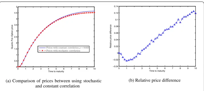
Figure 8 BS parameters:K= 80,S0= 100,R0= 1,rd= 0.05,re= 0.03,σS= 0.2,σR= 0.4, SCP
parameters:κ= 7.937,μ= 0.003,σ= 1.186 andρ0= 0.3.
We use a conditional Monte-Carlo approach and first simulate all the paths ofρi
t, for
i∈ {, , . . . ,M}and for each path we can compute a pricePi
Quantoby the pricing formula
(). Then the fair pricePis the mean value over all prices
P=E
E[PQuanto|Ft]
≈
M
i=PQuantoi
M . ()
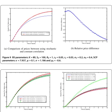
In Figure , we assume the parameter for the Black-Scholes model and use the estimated parameter for the SCP model (see Figure ). Besides, we apply the sample coefficient corre-lation () to estimate a constant correcorre-lation using the whole historical data (Jan -Mar ) of S&P and Euro/US-Dollar exchange rate, which is .. At the same time, we can let the SCP starting from the first correlation in the historical correlations. In Fig-ure b we present the relative difference between the price with constant correlation and stochastic correlation. We can observe, whilst the maturityTis shorter than three years, the prices with constant correlation are lower than the prices with stochastic correlation. However, for the contracts with maturities which are longer than three years, the prices using constant correlation are higher than the prices using stochastic correlation. The reason for this, for a short maturity (T< ), the SCP provides the correlations which are still closed to the initial correlationρ= ., which is larger than the constant correlation ρ= .. Since the price of quanto increases direct proportional with the correlation, therefore, the prices using stochastic correlation are higher than the prices using constant correlation for these short maturities. However, for the long maturities (T> ), the gener-ated correlations will tend to the mean reversion valueμ= . which are less than the value of the constant correlation, the prices with the constant correlation are thus higher. If we letρto be a value which is lower than the constant correlationρ= ., e.g. ρ= –.. And we choose a larger value forμ, say .. We can expect that the prices with
constant correlation will be higher than the prices with stochastic correlation only for the short maturities. For the longer maturities, the prices using stochastic correlations are higher, see Figures .
Figure 9 BS parameters:K= 80,S0= 100,R0= 1,rd= 0.05,re= 0.03,σS= 0.2,σR= 0.4, SCP
parameters:κ= 7.937,μ= 0.1,σ= 1.186 andρ0= –0.6.
Figure 10 BS parameters:K= 80,S0= 100,R0= 1,rd= 0.05,re= 0.03,σS= 0.2,σR= 0.4.
closed to each other forκ= . This is because that, for a large value ofκ, the correlation
tends rapidly to the mean reversion valueμof the SCP process. And the value ofμhas
been set to be equal to the value of constant correlation, the price differences are thus quite small.
In contrast, fixing a value for κ, the price differences between using constant and
stochastic correlation become bigger by increasing the value of the diffusionσ(and thus randomness in the SCP process), as shown in Figure b.
6 Conclusion
In this work we have revised concisely some stochastic correlation models. Market obser-vations give strong evidence that financial quantities are correlated in a strongly nonlin-ear, non-deterministic way. Instead of assuming a constant correlation, correlation has to be modelled as a stochastic process. We discussed first the general stochastic correlation model proposed in [] and proved that the stochastic correlation process in [] can be obtained by applying this general approach.
cor-relation. The numerical results showed that the correlation risk caused by using a wrong (constant) correlation model cannot be neglected.
Competing interests
The authors declare that they have no competing interests.
Authors’ contributions
All authors contributed to this paper as a whole. However, special merits go to LT for the idea and careful analysis; to ME for the introduction and MG for the application example. All authors read and approved the final manuscript.
Acknowledgements
The work of the authors was partially supported by the European Union in the FP7-PEOPLE-2012-ITN Programme under Grant Agreement Number 304617 (FP7 Marie Curie Action, Project Multi-ITNSTRIKE - Novel Methods in Computational Finance). Further the authors acknowledge partial support from the bilateral German-Spanish ProjectHiPeCa - High Performance Calibration and Computation in Finance, financed by DAAD.
Received: 16 November 2015 Accepted: 2 March 2016
References
1. Campbell JW, Lo AW, MacKinlay AC. The econometrics of financial markets. Princeton: Princeton University Press; 1997.
2. Brigo D, Chourdakis K. Counterparty risk for credit default swaps: impact of spread volatility and default correlation. Int J Theor Appl Finance. 2009;12:1007-26.
3. Teng L, Ehrhardt M, Günther M. Bilateral counterparty risk valuation of CDS contracts with simultaneous defaults. Int J Theor Appl Finance. 2013;16(7):1350040.
4. McNeil AJ, Frey R, Embrechts P. Quantitative risk management: concepts, techniques, and tools. Princeton: Princeton University Press; 2005.
5. Schöbel R, Zhu J. Stochastic volatility with an Ornstein-Uhlenbeck process: an extension. Eur Finance Rev. 1999;3:23-46.
6. Engle RF. Dynamic conditional correlation: a simple class of multivariate GARCH. J Bus Econ Stat. 2002;20(3):339-50. 7. Langnau A. Introduction into “local correlation” modelling. arXiv:0909.3441 (2009)
8. Gourieroux C, Jasiak J, Sufana R. The Wishart autoregressive process of multivariate stochastic volatility. J Econom. 2009;150:167-81.
9. Bowman AW, Azzalini A. Applied smoothing techniques for data analysis. New York: Oxford University Press; 1997. 10. van Emmerich C. Modelling correlation as a stochastic process. Preprint 06/03, University of Wuppertal (June 2006) 11. Ma J. Pricing foreign equity options with stochastic correlation and volatility. Ann Econ Financ. 2009;10(2):303-27. 12. Teng L, van Emmerich C, Ehrhardt M, Günther M. A versatile approach for stochastic correlation using hyperbolic
functions. Int J Comput Math. 2016;93(3):524-39.
13. Oksendal B. Stochastic differential equations. Berlin: Springer; 2000.
14. Uhlenbeck GE, Ornstein LS. On the theory of Brownian motion. Phys Rev. 1930;36:823-41. 15. Risken H. The Fokker-Planck equation. Berlin: Springer; 1989.
16. Wilmott P. Paul Wilmott on quantitative finance. 2nd ed. West Sussex: Wiley; 2006.