_______________
E-mail addresses: [email protected], [email protected]
Received November 17, 2017
373 Available online at http://scik.org
J. Math. Comput. Sci. 8 (2018), No. 3, 373-393 https://doi.org/10.28919/jmcs/3575
ISSN: 1927-5307
Numerical Computation of Some Iterative Techniques for Solving
System of Linear Equations of Multivariable
AZIZUL HASAN
Department of Mathematics, Faculty of Science, Jazan University, Jazan, KSA
Copyright © 2018 A Hasan . This is an open access article distributed under the Creative Commons Attribution License, which permits unrestricted use, distribution, and reproduction in any medium, provided the original work is properly cited.
Abstract:In this paper we introduce, numerical computation of some iterative techniques for solving system of linear simultaneous equations of 4 or more variables. Many iterative techniques is presented by the different formulae. Using
Jacobi method, Seidel method and SOR method and their results are compared. The software, Matlab 2009a was used
to find the solution of the linear simultaneous equations having diagonally dominant in coefficient matrix. Numerical
rate of convergence of solution has been found in each calculation. It was observed that the Seidel method converges
at the 12iteration while Jacobi and SOR methods converge to the exact value of X(x, y, z, t) with error level of accuracy
10−15 at the 22th iteration respectively. However, when we compare performance, we must compare both cost, speed of convergence. Some numerical examples are given to illustrate the efficiency and robustness of the techniques. It
was then concluded that Seidel is the most effective technique.
Keywords: iterative techniques; algorithm; linear simultaneous equations on large scale; rate of convergence; numerical experiments, executing time.
1.
Introduction
Solving system of linear simultaneous equations is one of the most important and challenging
problems in science and engineering applications. It arises in a wide variety of practical
applications in Physics, Chemistry, Biosciences, Engineering, etc. System of linear equations
arises in various theoretical research fields as well as applications in science and engineering. After
operations. Well known techniques of linear algebra such as Gaussian elimination and Gauss
Jordon’s methods are utilized to determine a common solution. Specifically, the problem of
existence, uniqueness and cardinality of solution of a system of linear equations is well solved in
linear algebra. In linear algebra, Iterative solver is an algorithm [1] that can be used to determine
the solutions of a system of linear equations to find the rank of a matrix [3-5], and to calculate the
inverse of an invertible square matrix. Another point of view, which turns out to be very useful to
analyze the algorithm. The first part of the algorithm computes an LU decomposition (it is a matrix
decomposition which writes a matrix as the product of a lower triangular matrix and an upper
triangular matrix. A linear equation system is a set of linear equations to be solved simultaneously.
This system consists of linear equations, each with coefficients, and has unknowns which have
to fulfill the set of equations simultaneously. To simplify notation, it is possible to rewrite the
equations in matrix notation which are diagonally dominant in coefficients matrix.[6-8] .Consider a system of n linear algebraic equations in n unknowns where (m=n)
𝑎11𝑥1 + 𝑎12𝑥2+ ⋯ … … . . 𝑎1𝑛𝑥𝑛 = 𝑏1 𝑎21𝑥1+ 𝑎22𝑥2 + ⋯ … … . . 𝑎2𝑛𝑥𝑛 = 𝑏2 … … … ….
𝑎𝑚1𝑥1+ 𝑎𝑚2𝑥2+ ⋯ … … . . 𝑎𝑚𝑛𝑥𝑛 = 𝑏𝑚 (i)
Where 𝑎𝑖𝑗, (𝑖, 𝑗 = 1(1)𝑛 are the known coefficient , 𝑏𝑖,(i = 1(1)n) are the known values and
𝑥𝑖 ,( i= 1(1)n) are the unknowns to be determined . In matrix notation the system can be written
as
A x = b (ii)
where A =
[
𝑎𝑎1121 𝑎𝑎1222 𝑎𝑎1323
… … … … … …
𝑎𝑚1 𝑎𝑚2 𝑎𝑚𝑛 ]
The matrix [ 𝐴 ∶ 𝑏] is called the augmented matrix. It is formed by appending the column b to the
𝑚×𝑛 matrix. The methods of solution of the linear algebraic equations (ii) may broadly be
classified into two types. (i) Direct methods: These methods produce the exact solution after a
finite number of steps. (ii) Iterative methods: These methods give a sequence of approximate
solutions, which converges when the number of steps tends to infinity. Here we are interested in
the case when m = n; particularly when the number of equations are large. A took-kit to solve
methods to solve equation (ii), we have to know the conditions under which the solutions exist.
We then proceed to develop direct and iterative methods for solving large scale problems. We later
discuss numerical conditioning of a matrix and its relation to errors that can arise in computing
numerical solutions.[6]
2.
Iterative Techniques
By this approach, we start with some initial guess solution, say 𝑥(0) , for solution x and generate an improved solution estimate 𝑥(𝑘+1)from the previous approximation x(k) .This method is a very
effective for solving differential equations, integral equations and related problems [4]. Let the
residue vector r be defined as
𝑟𝑖(𝑘) = 𝑏
𝑖 − ∑𝑛𝑗=1𝑎𝑖𝑗𝑥𝑗(𝑘) for i=1,2,…..n (3)
ie. r(k) = b − Ax(k) The iteration sequence {x(k): k = 0,1, … … } is terminated when some norm of the residue ‖r(k)‖ = ‖Ax(k) −b‖ becomes sufficiently small, ie.
‖𝑟(𝑘)
𝑏 ‖ < 𝜖 (4)
Where𝜖 is an arbitrarily small number as 𝜀 = 10−15another possible termination criterion can be
‖𝑥(𝑘)−𝑥(𝑘+1)
𝑥(𝑘+1) ‖ < 𝜖 (5)
It may be noted that the later condition is practically equivalent to the previous termination
condition. A simple way to form an iterative scheme is Richardson iterations [4]
x(k+1) = (I − A)x(k)+ b (6)
[4] Richardson iterations preconditioned with approximate inversion
x(k+1)= (I − MA)x(k)+ Mb (7)
Where matrix M is called approximate inverse of A if ‖I − MA‖ < 1 . A question that naturally arises is will the iterations converge to the solution of Ax = b. In this section, to begin with, some
well-known iterative schemes are presented. Their convergence analysis is presented next. In the
derivations that follow, it is implicitly assumed that the diagonal elements of matrix A are
non-zero, i.e.𝑎𝑖𝑖, ≠ 0, if this is not the case, simple row exchange is often sufficient to satisfy this
condition.
Theorem2.1. A matrix A is called strictly diagonally dominant if:
∑𝑛 |𝑎𝑖𝑗| < |𝑎𝑖𝑖|
Theorem2.2. A sufficient condition for the convergence of Jacobi and Gauss-Seidel methods is
that the matrix A of linear system Ax=b is strictly diagonally dominant [6]
Theorem.2.3. For any arbitrary matrix A, the necessary condition for the convergence of
relaxation method is 0 < w < 2. [9]
3. Materials and Methods
3.1. Jacobi-Method: Suppose we have a guess solution, say x(k)
x(k) = [𝑥1(𝑘) 𝑥
2(𝑘) 𝑥3(𝑘)… … … … 𝑥𝑛(𝑘)] T
for, Ax = b: To generate an improved estimate starting from x(k);consider the first equation in the
set of equations Ax = b, i.e.,
𝑎11𝑥1+ 𝑎12𝑥2+ ⋯ … … . . 𝑎1𝑛𝑥𝑛 = 𝑏1 (8) Rearranging this equation, we can arrive at a iterative formula for computing, x1(k+1), as
𝑥1(𝑘+1) = 1
𝑎11[𝑏1− 𝑎12𝑥2
(𝑘)… … . − 𝑎
1𝑛𝑥𝑛(𝑘)] (9)
Similarly, using second equation from Ax = b, we can derive
𝑥2(𝑘+1) = 1
𝑎22[𝑏2− 𝑎21𝑥1
(𝑘)− 𝑎
23𝑥3(𝑘)… … . − 𝑎2𝑛𝑥𝑛(𝑘)] (10)
In general, using ith row of Ax = b; we can generate improved guess for the ith element x of as follows
𝑥𝑖(𝑘+1) = 1
𝑎𝑖𝑖[𝑏2− 𝑎𝑖1𝑥1
(𝑘)… − 𝑎
𝑖,𝑖−1𝑥𝑖−1(𝑘)− 𝑎𝑖,𝑖+1𝑥𝑖+1(𝑘)… − 𝑎𝑖,𝑛𝑥𝑛(𝑘)] (11)
The above equation can also be rearranged as follows
𝑥𝑖(𝑘+1) = 𝑥𝑖(𝑘)+ (𝑟𝑖(𝑘)
𝑎𝑖𝑖 )
Where ri(k) is defined by equation (4). In matrix form, the method can be written as x(k+1)= −D−1(L + U)x(k)+ D−1b
The algorithm for implementing the Jacobi iteration scheme is summarized in Chart 1.
Chart 1: Algorithm for Jacobi Iterations
INITIALIZE: b, A, x(0) , kmax, 𝜖 k =0
𝛿 = 100 ∗ 𝜖
WHILE [(𝛿 > 𝜖) 𝐴𝑁𝐷 (𝑘 < 𝑘𝑚𝑎𝑥)]
𝑟𝑖 = 𝑏𝑖 − ∑𝑛𝑗=1𝑎𝑖𝑗𝑥𝑗 𝑥𝑁𝑖 = 𝑥𝑖 + ( 𝑟𝑖 𝑎𝑖𝑖) END FOR 𝛿 = ‖𝑟‖/‖𝑏‖ 𝑥 = 𝑥𝑁 k =k+1 END WHILE
3.2. Gauss-Seidel Method: When matrix A is large, there is a practical difficulty with the Jacobi
method. It is required to store all components of x(k) in the computer memory (as a separate
variables) until calculations of x(k+1) is over. The Gauss-Seidel method overcomes this difficulty
by using xi(k+1) immediately in the next equation while computing xi+1(k+1) :This modification leads to the following set of equations
𝑥1(𝑘+1) = 1
𝑎11[𝑏1− 𝑎12𝑥2
(𝑘)− 𝑎
13𝑥3(𝑘)… … . 𝑎1𝑛𝑥𝑛(𝑘)] (12)
𝑥2(𝑘+1)= 1
𝑎22[𝑏2− {𝑎21𝑥1
(𝑘+1)) } − {𝑎
23𝑥3(𝑘)+ ⋯ … . + 𝑎2𝑛𝑥𝑛(𝑘)}] (13)
𝑥3(𝑘+1) = 1
𝑎33[𝑏3− {𝑎31𝑥1
(𝑘+1))+ 𝑎
32𝑥2(𝑘+1)) } − {𝑎34𝑥4(𝑘)+ ⋯ … . + 𝑎3𝑛𝑥𝑛(𝑘)}] (14)
In general, for i’th element of x, we have
𝑥𝑖(𝑘+1) = 1
𝑎𝑖𝑖[𝑏𝑖− ∑ 𝑎𝑖𝑗𝑥𝑗
(𝑘+1)− ∑ 𝑎 𝑖𝑗𝑥𝑗(𝑘) 𝑛
𝑗=𝑖+1 𝑖−1
𝑗=1 ]
To simplify programming, the above equation can be rearranged as follows
𝑥𝑖(𝑘+1) = 𝑥
𝑖(𝑘)+ ( 𝑟𝑖(𝑘)
𝑎𝑖𝑖) (15)
where 𝑟𝑖(𝑘) = [𝑏𝑖 − ∑𝑖−1𝑗=1𝑎𝑖𝑗𝑥𝑗(𝑘+1)− ∑𝑛𝑗=𝑖+1𝑎𝑖𝑗𝑥𝑗(𝑘)]
In matrix form, the method can be written as
x(k+1)= −(L + D)−1Ux(k)+ (L + D)−1b (16)
The algorithm for implementing Gauss-Siedel iteration scheme is summarized in Chart2.
Chart 2: Algorithm for Gauss Seidel Iterations
INITIALIZE: b, A, x(0) , kmax, 𝜖 k =0
𝛿 = 100 ∗ 𝜖
FOR i =1 : n
𝑟𝑖 = 𝑏𝑖 − ∑𝑛𝑗=1𝑎𝑖𝑗𝑥𝑗
𝑥𝑖 = 𝑥𝑖 + ( 𝑟𝑖 𝑎𝑖𝑖) END FOR
𝛿 = ‖𝑟‖/‖𝑏‖
k =k+1
END WHILE
3.3. SUCESSASIVE OVER RELAXTION METHOD: Suppose we have a starting value say y,
of a quantity and we wish to approach a target value, say y* by some method. Let application of the method change the value from y to y^. If y^ is between y and y^ which is even closer to y than y*. Then we can approach y* faster by magnifying the change (y^ - y) [3]. In order to achieve this, we need to apply a magnifying factor w > 1 and get
𝑦∗= 𝑦 + 𝑤(y^ − y) (17)
This amplification process is an extrapolation and is an example of over-relaxation. If the
intermediate value y^ tends to overshoot target y*, then we may have to use w < 1; this is called under-relaxation. Application of over-relaxation to Gauss-Seidel method leads to the following set
of equations
𝑥𝑖(𝑘+1) = 𝑥𝑖(𝑘)+ 𝑤[𝑧𝑖(𝑘+1)− 𝑥𝑖(𝑘)] for i =1,2,…n (18) Where zi(k+1) are generated using the Gauss-Seidel method,
𝑧𝑖(𝑘+1)= 1
𝑎𝑖𝑖[𝑏𝑖 − ∑ 𝑎𝑖𝑗𝑥𝑗
(𝑘+1)− ∑ 𝑎 𝑖𝑗𝑥𝑗(𝑘) 𝑛
𝑗=𝑖+1 𝑖−1
𝑗=1 ] for i =1,2…n (19)
In matrix form, the method can be written as
x(k+1)= (wL + D)−1[(1 − w)D − wU]x(k)+ wb (20)
Thus, in general, an iterative method can be developed by splitting matrix A. The steps in the
implementation of the over-relaxation iteration scheme are summarized in Chart 3. It may be
noted that w is a tuning parameter, which is chosen such that 1 < w < 2 [9]
Chart 3: Algorithm for Gauss Seidel Iterations
INITIALIZE: b, A, x(0) , kmax, 𝜖 k =0
𝛿 = 100 ∗ 𝜖
FOR i =1 : n
𝑟𝑖 = 𝑏𝑖 − ∑𝑛𝑗=1𝑎𝑖𝑗𝑥𝑗
𝑧𝑖 = 𝑥𝑖 + (𝑟𝑖/𝑎𝑖𝑖)
𝑥𝑖 = 𝑥𝑖 + 𝜔(𝑧𝑖 − 𝑥𝑖)
END FOR
r = b - Ax
𝛿 = ‖𝑟‖/‖𝑏‖
k =k+1
END WHILE
3.4. Matlab Programs: Jacobi method, Gauss Seidel and SOR Methods are below as [10]
clc;
clear all;
% 3.112x + 0.5756y - 0.1565z - 0.0067t = 1.571
% 0.5756x + 2.938y + 0.1103z - 0.0015t = -0.9275
% -0.1565x + 0.1103y + 4.127z + 0.2015t = -0.06502
% -0.0067x - 0.0015y+ 0.2051z + 4.133t = -0.0177
A = [3.112 0.5756 -0.1565 -0.0067; 0.5756 2.938 0.1103 -0.0015; -0.1565 0.1103 4.127 0.2015 ;
-0.0067 -0.0015 0.2051 4.133];
b = [1.571; -0.9275; -0.06502; -0.0177];
% error tolerance
tol = 0.000000000000005;
%initial guess:
x0 = zeros(n,1); here n=4
% Jacobi method
%---
xnew=x0;
error=1;
while error>tol
xold=xnew;
off_diag = [1:i-1 i+1:length(xnew)];
xnew(i) = 1/A(i,i)*( b(i)-sum(A(i,off_diag)*xold(off_diag)) );
end
error=norm(xnew-xold)/norm(xnew);
end
x_jacobian=xnew
%Gauss Seidel Method:
%---
maxiter=1000;
lambda=1;
n=length(x0);
x=x0;
error=1;
iter = 0;
while (error>tol & iter<maxiter)
xold=x;
for i=1:n
I = [1:i-1 i+1:n];
x(i) = (1-lambda)*x(i)+lambda/A(i,i)*( b(i)-A(i,I)*x(I) );
end
error = norm(x-xold)/norm(x);
iter = iter+1;
end
x_siedal=x
%SOR
%---
maxiter=1000;
lambda=1.2;
n=length(x0);
x=x0;
iter =0;
while (error>tol & iter<maxiter)
xold=x;
for i=1:n
I = [1:i-1 i+1:n];
x(i) = (1-lambda)*x(i)+lambda/A(i,i)*( b(i)-A(i,I)*x(I) );
end
error = norm(x-xold)/norm(x);
iter = iter+1;
end
4.
Convergence Analysis of Iterative Methods
The convergence analysis can be carried out if the above set of iterative equations are expressed
in the vector-matrix notationTo discuss the convergence of the iterative methods (ii) .we study
the behavior of the difference between the exact solution x and an approximate 𝑥(𝑘). The exact solution x will satisfy
𝑥 = 𝐻𝑥 + 𝑐 (21)
Where H = ‖I − MA‖ < 1 , Subtracting (21) from (6) and substituting 𝜖(𝑘)= 𝑥(𝑘)− 𝑥 , we get 𝜖(𝑘+1) = 𝐻𝜖(𝑘) , k = 0,1, 2 ,………
From which we obtain 𝜖(𝑘)= 𝐻(𝑘)𝜖(0) k = 0, 1, 2,……….
Where we have assumed that the iteration matrix H remains constant for each iteration.We given
few results above which we require for providing the convergence of the iterative methods.[1 ]
5.
Numerical Experiments and Comparative discussion
In this section, we employ the various techniques obtained in this paper to solve system of linear
simultaneous equations and compare them. We use the stopping criteria |𝑥𝑘+1− 𝑥𝑘| < 𝜀 and
|𝑓(𝑥𝑘+1)| < 𝜀, where 𝜀 = 10−15 , for computer programs. All programs are written in
Matlab2009a .The results are presented in Table1to3. Example1. Let us consider the system of
3.112x +0.5756y -0.1565z -0.0067t =1.5710
0.5756x + 2.938y + 0.1103z - 0.0015t =-0.9275
-0.1565x + 0.1103y + 4.127z + 0.2015 t= -0.06502 -0.0067x - 0.0015y + 0.2051z + 4.133 t = - 0.0177
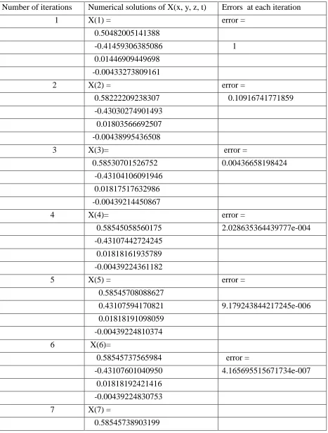
Table1. Numerical Solutions of Iteration data for Jacobi method, with 𝜀 = 10−15 Number of iterations Numerical solutions of X(x, y, z, t) Errors at each iteration
1 X(1) = error =
0.50482005141388
-0.31569094622192 1
-0.01575478555852
-0.00428260343576
2 X(2) = error =
0.56240918742365
-0.41400377557926 0.16792158814306
0.01203489072131
-0.00279698416569
3 X(3) = error =
0.58199398901909
-0.42632892178484 0.03278271009799
0.01677374523566
-0.00411836927040
4 X(4) = error =
0.58450913413709
-0.43034447302001 0.00671700306133
0.01791034426032
-0.00432625908640
5 X(5) = error =
0.58530856735578
-0.43088000611636 0.00135749643692
-0.00438004285473
6 X(6) = error =
0.58541820851009
-0.43104464587601 2.799561402866404e-004
0.01817044683815
-0.00438950385209
7 X(7) = error =
0.58545101652333
-0.43106790516012 5.675417343725499e-005
0.01817946670660
-0.00439173085369
8 X(8)= error =
0.58545576740136
-0.43107467252718 1.170187868812868e-005
0.01818144119023
-0.00439213372092
9 X(9) = error =
0.58545711753116
-0.43107567763107 2.376226925696227e-006
0.01818182188583
-0.00439222645907
10 X(10) = error =
0.58545732238184
-0.43107595648218 4.896841447296750e-007
0.01818190447488
-0.00439224352716
11 X(11)= error =
0.58545737807514
-0.43107599972494 9.957377583570863e-008
-0.00439224739476
12 X(12) = error =
0.58545738687241
-0.43107601124081 2.050878105103282e-008
0.01818192398557
-0.00439224811686
13 X(13) = error =
0.58545738917467
-0.43107601309447 4.175149479277625e-009
0.01818192466221
-0.00439224827831
14 X(14) = error =
0.58545738955120
-0.43107601357100 8.594936849327012e-010
0.01818192480694
-0.00439224830883
15 X(15) = error =
0.58545738964656
-0.43107601365022 1.751459502654988e-010
0.01818192483544
-0.00439224831557
16 X(16) = error =
0.58545738966263
-0.43107601366997 3.603792102737823e-011
0.01818192484151
-0.00439224831686
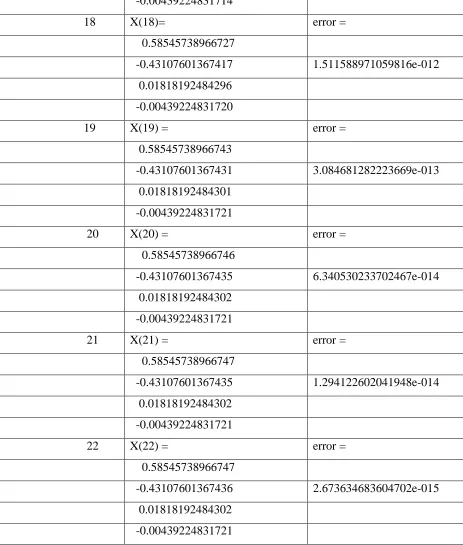
17 X(17) = error =
0.58545738966658
-0.43107601367335 7.349898927456906e-012
-0.00439224831714
18 X(18)= error =
0.58545738966727
-0.43107601367417 1.511588971059816e-012
0.01818192484296
-0.00439224831720
19 X(19) = error =
0.58545738966743
-0.43107601367431 3.084681282223669e-013
0.01818192484301
-0.00439224831721
20 X(20) = error =
0.58545738966746
-0.43107601367435 6.340530233702467e-014
0.01818192484302
-0.00439224831721
21 X(21) = error =
0.58545738966747
-0.43107601367435 1.294122602041948e-014
0.01818192484302
-0.00439224831721
22 X(22) = error =
0.58545738966747
-0.43107601367436 2.673634683604702e-015
0.01818192484302
-0.00439224831721
Table 1 shows that the iteration data obtained for Jacobi method .it is observed that the numerical
Solutionof the linear simultaneous equation converges at 22 iteration with error level of
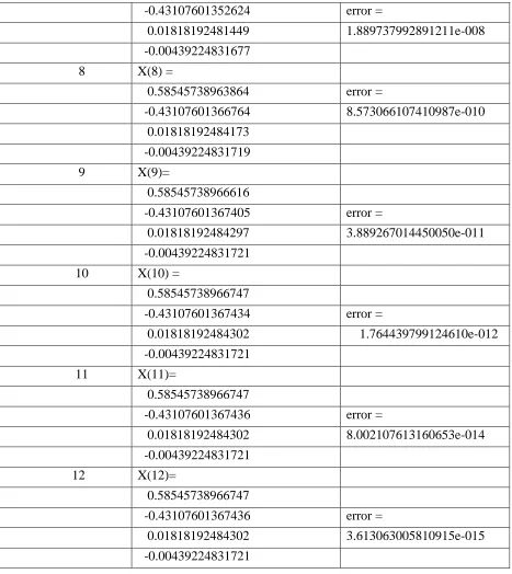
Table 2. Numerical Solutions of Iteration data for Gauss Seidel method, with 𝜀 = 10−15
Number of iterations Numerical solutions of X(x, y, z, t) Errors at each iteration
1 X(1) = error =
0.50482005141388
-0.41459306385086 1
0.01446909449698
-0.00433273809161
2 X(2) = error =
0.58222209238307 0.10916741771859
-0.43030274901493
0.01803566692507
-0.00438995436508
3 X(3)= error =
0.58530701526752 0.00436658198424
-0.43104106091946
0.01817517632986
-0.00439214450867
4 X(4)= error =
0.58545058560175 2.028635364439777e-004
-0.43107442724245
0.01818161935789
-0.00439224361182
5 X(5) = error =
0.58545708088627
0.43107594170821 9.179243844217245e-006
0.01818191098059
-0.00439224810374
6 X(6)=
0.58545737565984 error =
-0.43107601040950 4.165695515671734e-007
0.01818192421416
-0.00439224830753
7 X(7) =
-0.43107601352624 error =
0.01818192481449 1.889737992891211e-008
-0.00439224831677
8 X(8) =
0.58545738963864 error =
-0.43107601366764 8.573066107410987e-010
0.01818192484173
-0.00439224831719
9 X(9)=
0.58545738966616
-0.43107601367405 error =
0.01818192484297 3.889267014450050e-011
-0.00439224831721
10 X(10) =
0.58545738966747
-0.43107601367434 error =
0.01818192484302 1.764439799124610e-012
-0.00439224831721
11 X(11)=
0.58545738966747
-0.43107601367436 error =
0.01818192484302 8.002107613160653e-014
-0.00439224831721
12 X(12)=
0.58545738966747
-0.43107601367436 error =
0.01818192484302 3.613063005810915e-015
-0.00439224831721
Table 2 shows that the iteration data obtained for Gauss Seidel method .it was observed that the
numerical Solutionof the linear simultaneous equation converges at the 12 iteration with error
Table3. Numerical Solutions of Iteration data for SOR method, with 𝜀 = 10−15
No. of iterations Numerical Solutions of X(x,y,z,t) Errors in each iterations
1 X(1) =
0.60578406169666 error =
-0.52124818485198 1
0.02537791532194
-0.00569894880129
2 X(2) =
0.60183698560092 error =
-0.41721738878662 0.14258422119967
0.01712017300438
-0.00402978171698
3 X (3)=
0.57904235989393 error =
-0.43229151833930 0.03783623815512
0.01812010442860
-0.00447406888318
4 X(4) =
0.58700623934679
-0.43119431035112 error =
0.01827335748195 0.01103642226787
-0.00437836752937
5 X (5)=
0.58517942967110 error =
-0.43099111693600 0.00253429231144
0.01814745363045
-0.00439347546181
6 X(6) =
0.58549205511306 error =
0.01819122459500
-0.00439249952107
7 X(7) =
0.58545625013082 error =
-0.43107144950102 6.453339771903484e-005
0.01817988137485
-0.00439207661696
8 X(8) =
0.58545648166585 error =
-0.43107144950102 7.863608435704243e-006
0.01817988137485
-0.00439207661696
9 X(9) =
0.58545772862405 error =
-0.43107662087342
0.01818230163190 2.015299667709794e-006
-0.00439230712583
10 X(10) =
0.58545731296901 error =
-0.43107598893356 5.789747813536638e-007
0.01818186756164
-0.00439223247423
11 X(11) =
0.58545740191311 error =
-0.43107599800051 1.264805602506763e-007
0.01818193137820
-0.00439225201736
12 X(12) =
0.58545738860102 error=
0.01818192451241
-0.00439224753642
13 x(13)=
0.58545738953652 error =
-0.43107601214618 2.803660810121424e-009
0.01818192476586
-0.00439224847019
14 X(14) =
0.58545738975562 error =
-0.43107601394582 5.189434870315965e-010
0.01818192487017
-0.00439224828861
15 X(15) =
0.58545738964239 error =
-0.43107601364199 1.624058027681464e-010
0.01818192483889
-0.00439224832250
16 X(16) =
0.58545738967258 error =
-0.43107601367475 4.154743530371315e-011
0.01818192484303
-0.00439224831621
17 X(17) =
0.58545738966671 error =
-0.43107601367548 8.346869132251461e-012
0.01818192484323
-0.00439224831742
18 X(18) =
0.58545738966753 error =
0.01818192484295
-0.00439224831717
19 X(19) =
0.58545738966748 error =
-0.43107601367445 1.633847938958885e-013
0.01818192484304
-0.00439224831722
20 X(20) =
0.58545738966746
-0.43107601367434 error =
0.01818192484302 3.043187461809806e-014
-0.00439224831721
21 X(21) =
0.58545738966747 error =
-0.43107601367436
0.01818192484302 9.427901987222536e-015
-0.00439224831721
22 X(22)=
0.58545738966747 error =
-0.43107601367436
0.01818192484302 2.297594335026736e-015
-0.00439224831721
Table 3 shows that the iteration data obtained for SORmethod .it was observed that the
numerical Solutionof the linear simultaneous equation converges at the 22 iteration with error
Example-2 Let us consider another the system of linear simultaneous equations of n=5 variables
10 v + w+ x – 2y + z =-1 , v- 20 w - 2x + y + z = 20 , v + w + 10 x –y – z = 1
-v + 2w + x + 50 y + z = 2 , v + w + x + y +100 z =- 1
The solution of above equations are converges 16, 11, 24 iterations respectively by the above
techniques up to error level of 𝜀 = 10−15 which are given below.
v = -0.00364280090102
w = -1.01743940692132
x = 0.20949210878712
y= 0.07648785763481
z = -0.00264897758600
Thus we can solve the system of linear simultaneous equations of more variable which are
diagonally dominant in coefficient matrix by the above techniques.
5.1. Executing time: The execution time of a given task is defined as the time spent by the system
executing that task, including the time spent executing run time or system services on its behalf.
Table 4: Execution time comparison for iterations data of various techniques
S/No.
Techniques
Number of iterations (Elapsed time)
Example1 Example2 Example1 Example2
1. Jacobi 22 16 0.015000 0.02000
2. Seidel 12 11 0.000140 0.01500
3. SOR 22 24 0.016000 0.02500
Thus from the above discussions we see that the Jacobi and SOR method is taking more time in
comparison to that of Seidel method to run the program. [11]. SOR method has more error than
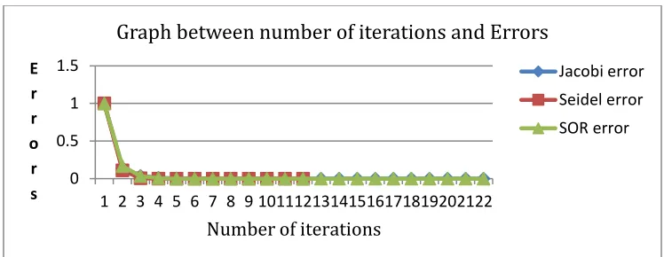
other Since the Seidel method requires less number of iterations and Jacobi and SOR method 0
0.5 1 1.5
1 2 3 4 5 6 7 8 9 10111213141516171819202122
E r r o r s
Number of iterations
Graph between number of iterations and Errors
required more iterations with error level 0.000000000000005 with optimal factor w = 1.2 Thus we
see that the overall performance of the iterative techniques are in this manner.
SOR method ≤ Jacobi method < Gauss Seidel method
CONCLUSION
The above plot is shows the result obtained from different algorithm. Consequently, we can see
that Gauss Seidel Technique is more accurate at large scale with different parameters such as
running time factor and number of iterations and error level. Based on our results and discussions,
we now conclude that the Seidel method is formally the most effective of the Jacobi and SOR
method, we have considered here in the study. Analysis of efficiency from the numerical
computation shows that Jacobi and SOR method converges slowly. Thus these methods have great
practical utilities. One can easily adopt these MATLAB codes as needed for a different type of
problem linear simultaneous equations of more order like 6×6 and so on. And also can use linear simultaneous differential equation for equilibrium problem in applied mathematics.
Conflict of Interests
The authors declare that there is no conflict of interests.
REFERENCES
[1] M.K.Jain, S.R.K. Iyenger and R.K.Jain. Numerical methods for scientific and engineering computation. New Age
International Publishers,147-154, 2010.
[2] Gourdin, A. and M Boumhrat; Applied Numerical Methods. Prentice Hall India, New Delhi.
[3] Strang, G.; Linear Algebra and Its Applications. Harcourt Brace Jovanovich College Publisher, New York, 1988.
[4] Kelley, C.T.; Iterative Methods for Linear and Nonlinear Equations, Philadelphia: SIAM, 1995.
[5] The MathWorks Inc. MATLAB: 7.8. or 2009a.
[6] Atkinson, K. E.; An Introduction to Numerical Analysis, John Wiley, 2001.
[7] Steven C. Chapra. Applied Numerical methods with matlab for engineers and scientist.2012
[8] Phillips, G. M. and P. J. Taylor; Theory and Applications of Numerical Analysis, Academic Press, 1996.61
[9] Sachin C. Patwardhan, Numerical Analysis Module 4 Solving Linear Algebraic Equations, Dept. of Chemical
Engineering, Indian Institute of Technology, Bombay, India.
[10] Bazara, M.S., Sherali, H. D., Shetty, C. M., Nonlinear Programming, John Wiley, 1979.