A Comparative Analysis of two Controllers for Trajectory Tracking Control: Application to a Biological Process

(1)

www.astesj.com

Special Issue on Multidisciplinary Sciences and Engineering

A Comparative Analysis of two Controllers for Trajectory

Tracking Control: Application to a Biological Process

Abyad Mohamed*, Karama Asma, Khallouq Abdelmounaim

LAEPT-URAC 28, Faculty of Science Semlalia, Cadi Ayyad University, Marrakech, Morocco

A R T I C L E I N F O A B S T R A C T

Article history:

Received: 01 June, 2018 Accepted: 04 August, 2018 Online: 20 August, 2018 Keywords:

Bioprocess Constraints Fuzzy observer LMIs

Takagi-Sugeno Model Trajectory tracking

The aim of the present work is to guarantee the trajectory tracking of a nonlinear biological process and compare two control approaches. The main objective of this work is to elaborate a fuzzy model and build a fuzzy controllers for a biological process by using the fuzzy Takagi-Sugeno. Two controllers are synthesized, the parallel distributed compensation control and optimal fuzzy linear quadratic integral control. In both cases, the physical constraints on the manipulated inputs are respected. In addition, the case with and without the observer is presented, where a fuzzy observer based control is used with unmeasurable premise variables. Finally, the performances and the effectiveness of both the modeling and the control are demonstrated via simulations.

1 Introduction

Nowadays, the biological processes become one of the important industrial processes thanks to their advan-tages, such as the treatment of organic substrates, pro-tein production and the production of ethanol gas etc. However, their modeling and control form a real chal-lenge problem for both control engineers and theorists, where this kind of systems are characterized by strong variations of system parameters and unknown kinetics owing to the time-varying characteristics and multiple interactions generated by the living microorganisms [1, 2]. Therefore, we obtain a highly nonlinear system. The motivation of this work is to linearize the model and benefit from linear theory control and to try to de-velop a nonlinear control, which is very difficult in this case. Also to use the Takagi-Sugeno (T-S) model, fur-thermore, the proposed controllers can be applied to the real process. It only needs to identify a T-S model from experimental data. T-S approach has been rec-ognized as an effective tool for handling the previous difficulty.

There are different techniques for controlling the bioprocess using Takagi-Sugeno models, such as opti-mal fuzzy linear quadratic regulators for discrete-time [3], a fuzzy integral controller to force the switching of a bioprocess between two different metabolic states is

treated in [4], an internal model control design strategy is developed for a particular Continuous Stirred-Tank Reactor (CSTR)[5]. A PID and fuzzy controller are pro-posed in [6] to stabilize the CSTR around the equilib-rium point, where the authors consider only one input, which is not the case in practice. Also, the case of un-certain Takagi-Sugeno system is treated in [7], where an observer with unmeasurable premise variables and unknown input is considered for a wastewater treat-ment plant. In addition, the predictive control based on fuzzy observer is studied for a sludge depollution bioprocess in [8, 9], in this framework one can cite [10, 11, 12]. Furthermore, the modeling and the con-trol of bioprocess based on neural network approach is treated in [13, 14]. In the same spirit, a nonlin-ear model autoregressive with exogenous input model predictive control is developed in [15] to control the fermentation process. Also, an integral backstepping control law is developed in [16] for controlling the dissolved oxygen level for bacteria fermentation.

The problem treated in this paper is how to model and control the biomass growth process, ensuring the trajectory tracking while taking into account the fol-lowing constraints:

- The mathematical model is nonlinear and not affine in control.

- The variables control present the physical constraints,

*_{Corresponding Author: Abyad Mohamed, Faculty of Science}

Semlalia Marrakech , Morocco, [email protected]

(2)

which make the computation of the control gains diffi -cult.

- The full system states are not measurable.

The present paper has two goals, the first is to build a fuzzy model of biological process based on Takagi-Sugeno tool, especially the nonlinearity sector meth-ods. The second is to ensure the tracking trajectory of the desired outputs using two approaches: the Par-allel Distributed Compensation (PDC) [17] and the Linear Quadratic Integral (LQI) control. Where the strong physical constraints on the inputs [18] are tak-ing into account. In addition, the proposed controllers are compared. The stability conditions are formed in the Linear Matrix Inequalities (LMIs) terms.

This paper is organized as follows: Section 2 presents the description of the Takagi-Sugeno mod-eling. Section 3 describes the parallel distributed com-pensation control. Then, one can address the fuzzy output tracking control problem in section 4 and we show that it can be solved by using two methods: the PDC technique and the optimal linear quadratic con-trol. Section 5 describes the controller design based on fuzzy observer with unmeasurable premise vari-ables. Section 6 introduces the proposed biological process. Finally, the simulation and the discussion of the obtained results are given to compare the proposed controllers.

2 Takagi-Sugeno Fuzzy Model

In order to extend the existing approaches of control and observation for linear to nonlinear system, Takagi and Sugeno have proposed a fuzzy dynamic model to represent this kind of system. The T-S fuzzy model is a set of linear models connecting via membership functions. To build the T-S fuzzy model, three methods exist in the literature [17]: The black box identification, the linearization method and the nonlinearity sector methods. The third method gives an exact T-S rep-resentation of nonlinear system without information loss.

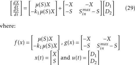
Consider the following nonlinear system:

˙

x(t) =f(x(t)) +g(x(t))u(t)

y(t) =Cx(t) (1)

where x∈Rnis the state, u∈Rm is the input vector,

y∈Rqrepresents the output measurement vectors and

C∈Rq∗nis the output matrix. In addition,f(.) andg(.) represent the nonlinear functions.

The T-S fuzzy model uses a set of fuzzy if-then rules, which represent local linear input-output relations of a nonlinear system. Theithrule of the T-S model given as follows:

Rule i:

ifz1(t) isF1i(z1(t))andz2(t) isF2i(z2(t)) ...andzp(t) is

Fip(zp(t))

Then

      

˙

x(t) =Aix(t) +Biu(t)

y(t) =Cix(t)

(2)

WhereF_pi are the membership functions of fuzzy sets,

i ∈ {₁_,₂_{, ...r}}_, _r _{is the number of rules,} _A_i ∈ Rn∗n,

Bi ∈Rn∗m,C_i∈Rq∗nandz₁(t), ..., z_p(t) are the premise variables which can be dependent of the input, the out-put or the state. The global T-S fuzzy model is given in the following form:

˙

x(t) = Pr

i=1

hi(z(t))(Aix(t) +Biu(t))

y(t) =Cx(t)

(3)

where

hi(z(t)) =

Qp

j=1Fji(zj(t)) r

P

i=1

Qp

j=1Fji(zj(t))

(4)

The activation functions hi(z(t)) indicates the acti-vation degree of theith associated local model, this functions verifies all time the convex sum propriety:

        

0≤_h_i₍_z₍_t₎₎≤₁

r

P

i=1

hi(z(t)) = 1,∀i∈ {1,2, ..., r}.

(5)

3 PDC control approach

3.1 Fuzzy regulator design via PDC

To stabilize the system presented by their T-S fuzzy model, the PDC controller is usually used to design a fuzzy controller. The main idea is to design a local con-troller for each sub-model based on local control rule, which shares with the fuzzy model the same fuzzy sets. The overall fuzzy controller is represented by:

u(t) =−

r

X

i=1

hi(z)Kix(t) (6)

Where theKi represent the local feedback gains. by using (6) in (3) the system in closed-loop becomes:

˙

x(t) = Pr

i=1 r

P

j=1

hi(z)hj(z)(Ai−BiKj)x(t)

= Pr

i=1

h2_i(z)Giix(t) + 2 r

P

i<j

hi(z)hj(z)( Gij+Gji

2 )x(t)

(7) withGij=Ai−BiKj, the stability conditions of (7) are given by the following theorem [17].

Theorem 1 The continuous fuzzy system(7)is asymp-totically stable, if there exist a common positive matrix

P ∈ _Rn×n _{and a common positive semi definite matrix}

Q ∈ _Rn×n _{and for a number of active rules} _s_{, where}

1< s≤_r_{such that:}

G_iiTP+P Gii+ (s−1)Q <0 (8)

(Gij+Gji

2 )

T_P₊_P₍Gij+Gji

2 )−Q≤0, i < j (9)

(3)

In order to transform the preview conditions into LMIs form, one can consider the following variables:X=P−1

, Ki =MiX −₁

, Q = P Y P, where X > 0, Y ≥ _{0 and}

Mi(i = 1, ..., r), then the stabilization conditions be-come:

AiX−BiMi+XATi −MiTBTi + (s−1)Y <0

AiX−BiMj+XATi −MjTBTi +AjX−BjMi +XAT_j −_MT

i BTj −2Y≤0, i < j

(10)

4 Trajectory tracking control

The trajectory tracking control of nonlinear systems is the subject this section. In the tracking loop, we con-sider the integral of the tracking erroreI=

R

(yr−y)dt=

R

(yr−Cx)dt[19], withyris the desired output. If we consider the following augmented state:

Xa=

"

x eI

#

Then, the following augmented system is obtained:

        

˙

Xa(t) = r

P

i=1

hi(z(t))( ¯AiXa(t) + ¯Biu(t) + ¯DYr)

y(t) = ¯CXa(t)

(11)

where: ¯Ai =

"

Ai 0

−_C ₀

#

, ¯Bi =

"

Bi 0

#

, ¯C=hC 0i, ¯D=

"

0 I

#

,

Yr=

"

yr1

yr2

#

withYr, denote the desired reference trajectory.

4.1 PDC control

To achieve the output tracking, the state feedback PDC control based on the previous LMIs can be used. The fuzzy controlleru(t) has the same form of (6), wherex

is replaced by the augmented stateXa:

u(t) =−

r

X

i=1

hi(z)KiXa(t) =− r

X

i=1

hi(z)(Ki xx+Ki IeI)

(12) The feedback gains of the controllerKi =

h

K_{i x} K_{i I}i

are obtained by solving the LMIs (10).

4.2 LQI control

To design the LQI control, the following quadratic cost criterion must be minimized by the control lawu(t):

J=

Z∞

0

(X_aT(t)QXa(t) +uT(t)Ru(t))dt (13)

for this reason, the following candidate quadratic Lya-punov function is considered:

V(Xa) =XaTP Xa (14)

The augmented system (7) is stable if :

XaTQXa+uTRu+ ˙V(Xa)<0 (15)

( ¯Ai+ ¯BiKi)TPi+Pi( ¯Ai+ ¯BiKi) +Q+KiTRKi<0 (16) ( ¯AiXi+ ¯BiYi)T+( ¯AiXi+ ¯BiYi)+XiQXi+YiTRYi <0 (17) ( ¯AiXi+ ¯BiYi)T + ( ¯AiXi+ ¯BiYi) +YiTRYi−Xi(−Q)Xi<0

(18) by using the Schur complement procedure, the follow-ing stability conditions are obtained:

       

¯

(AiXi+ ¯BiYi)T + ( ¯AiXi+ ¯BiYi) Xi YiT

∗ −_Q˜ ₀

∗ ∗ −_R˜

       

<0 (19)

where: Q−1 = ˜Q, R−1 = ˜R, Xi = P −₁

i , Ki = YiX −₁ i ,

i= 1, ..., r

This LMIs will be calculated for each sub-model, here is about the conventional linear quadratic integral con-trol using the fuzzy model. The concon-trol law is not based on fuzzy rules.

The control law will be respect the physical con-straints on the control input, where this problem is studied in many practical cases [20, 21, 22, 23]. To ensure the stabilization under constraints on the in-puts, the conditions given in the following theorem [17] must be verified.

Theorem 2 For a known initial conditionXa(0), the con-straint k_u₍_t₎k

2 ≤ η is enforced at all timest ≥0 if the LMIs:

"

1 Xa(0)T

Xa(0) X

#

≥₀ ₍₂₀₎

"

X M_iT Mi η2I

#

≥₀ ₍₂₁₎

hold

4.3 Observer design

In bioprocess control problems, the state variables are not usually available. By introducing the observer, one can reconstruct partially or all the state variables. This section presents the fuzzy observer design with unmea-surable premise variablesz(t) (hi(z),hi( ˆz)).

Based on the structure of the fuzzy model (3), the fuzzy observer is given as follows:

            

˙ˆ

x(t) = Pr

i=1

hi( ˆz)(Aixˆ(t) +Biu(t) +Li(y(t)−yˆ(t))

ˆ

y(t) =Pr

i=1

hi( ˆz)Cixˆ(t)

(22) where ˆxdenotes the estimated state andLi the gains of the observer.

In order to compute this gains the following theorem [24] gives the necessary conditions for ensuring the convergence of the state estimation error to zero.

Theorem 3 If there exist symmetric and definite positive matricesP ∈Rn×n,Q∈Rn×n, matricesY_i ∈Rn×qand a

scalarα >0such that:

AT_i P +P Ai−CTYiT −YiTC≤ −Q (23)

"

Q−_α2I P

P I

#

(4)

then, the estimation error between the T-S fuzzy model(3)

and the fuzzy observer(22)is converges asymptotically to zero.

where:Li=P −₁

Yi. Proof 1 See Appendix.

5 Process description

The proposed biological process in this paper is a biomass growth process, which consists to grow the population of microorganisms (biomass) by the con-sumption of a substrate (glucose), according to the following reaction scheme:

k1S µ(.)

7−→_X ₍₂₅₎

The dynamic model of this process is established from the mass-balance [25], which describes the evolution of substrate and biomass concentrations in a continuous bioreactor. This model can be represented by a high nonlinear system as follows:

      

dX

dt =µ(.)X−DX dS

dt =−k1µ(.)X+D(Sin−S)

(26)

The state variables are the biomassXand substrateS

concentrations,k1denotes the pseudo stoichiometric

coefficient andµ(.) represent the specific growth rate, the ”Monod law” characterizesµ(.) is:

µ(S) =µmax

S Ks+S

(27)

whereµmaxis the maximum specific growth rate;Ksis the Monod or saturation constant. The input variables are the dilution rateD(t) and the influent substrate concentrationSin. The parameters of the proposed model are given in the Table 1.

Parameters Value Unit

µmax 0.38 h −₁

Ks 5 g/l

k1 1/0.07

S_inmax 140 g/l

Table 1:Simulation parameters

5.1 Takagi-Sugeno model design

The model (26) must be transformed into affine in con-trol model like in (1), where the bioprocess models are known belong to the class of affine nonlinear models, this can be easily shown by assuming that:

D = D1+D2

Sin = D1D+2D2S max in

(28)

whereD1(t) andD2(t) are respectively the water and

the substrate dilution rate, then one can replaceD(t)

andSin(t) in (26) by their expressions (28), the follow-ing affine model is obtained:

"_dX

dt dS dt

#

=

"

µ(S)X

−_k₁_µ₍_S₎_X #

+

"

−_X −_X

−_S _Smax

in −S

# "

D1

D2

#

(29)

where:

f(x) =

"

µ(S)X

−_k₁_µ₍_S₎_X #

,g(x) =

"

−_X −_X

−_S _Smax

in −S

#

x(t) =

"

X S

#

andu(t) =

"

D1

D2

#

To build the T-S model, the following nonlinearities are considered:

z1(x) =µ(S) (30)

z2(x) =X (31)

z3(x) =S (32)

This leads:

A(z) =

"

z1 0

−_k₁_z₁ ₀ #

andB(z) =

"

−_z₂ −_z₂ −_z₃ −_z₃₊_Smax

in

#

where the number of nonlinaritiesn= 3, the global model can be represented byr= 2n = 8 sub-models. The local membership functions are defined by:

F1₁(z1) = z1 −_zmin

1 zmax

1 −z1min

, F2₁(z1) = z max 1 −z1 zmax

1 −zmin1

F1₂(z2) = z2−zmin2 zmax₂ −_zmin

2

, F2₂(z2) = z₂max−_z₂ zmax₂ −_zmin

2

F1₃(z3) = z3−zmin3 zmax

3 −z3min

, F2₃(z3) = zmax

3 −z3 zmax

3 −zmin3

Finally, the activation functions are:

h1(z) =F11(z1)F21(z2)F13(z3), h2(z) =F11(z1)F21(z2)F32(z3)

For the simulation, the parameters given in Table 1 are considered and leads to the followingminandmaxof premise variables:

0.018 ≤_µ₍_S₎≤₀_.₃₅

3.8 ≤_X≤₂₀

0.6 ≤_S≤₁₄₀

the computed matrixAi andBi of each sub-model are given as follows:

A1=A3=A5=A7=

"

0.3507 0

−₅_.₀₁₀₆ ₀ #

A2=A4=A6=A8=

"

0.0179 0

−₀_.₂₅₅₁ ₀ #

B1=B2=

"

−₂₀ −₂₀

−₁₄₀ ₀

#

, B3=B4=

"

−₃_.₈ −₃_.₈

−₁₄₀ ₀

#

B5=B6=

"

−₂₀ −₂₀

−₀_.₆ ₁₃₉_.₄ #

, B7=B8=

"

−₃_.₈ −₃_.₈ −₀_.₆₀ ₁₃₉_.₄

(5)

6 Simulation and results

In the first case, all the states variables (substrate and biomass concentrations) are supposed measurable (i.e.

C=

"

1 0

0 1

#

).

The desired trajectory (Xr andSr), which represent re-spectively of biomass and substrate concentrations are computed by using the following reference model:

˙

Xr=−0.97Xr+ 0.97refX ˙

Sr=−0.65Sr+ 0.65refS (33)

whererefXandrefS are the setpoints.

6.1 Tracking control based on state

feed-back

6.1.1 PDC control

The studied bioprocess presents the physical con-straints on the control as shown in the Table 2

Variables Constraints

Dilution rateh−1 0.016_D6₀_.₃₈

Influent substrateg/l 606_S_in6₁₄₀

Table 2:The control constraints

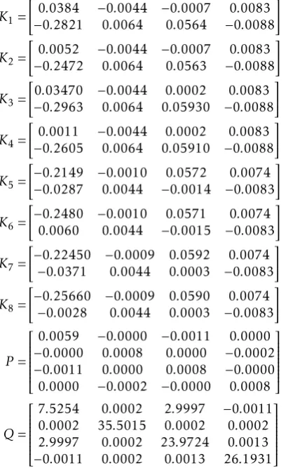
For a number of active sub-models= 5 andη = 1.55, the LMIs (10), (20) and (21) are solved by using the solver SeDuMi in MATLAB toolbox YALMIP, gives the following gains:

K1=

"

0.0384 −₀_.₀₀₄₄ −₀_.₀₀₀₇ ₀_.₀₀₈₃ −₀_.₂₈₂₁ ₀_.₀₀₆₄ ₀_.₀₅₆₄ −₀_.₀₀₈₈

#

K2=

"

0.0052 −₀_.₀₀₄₄ −₀_.₀₀₀₇ ₀_.₀₀₈₃ −₀_.₂₄₇₂ ₀_.₀₀₆₄ ₀_.₀₅₆₃ −₀_.₀₀₈₈

#

K3=

"

0.03470 −₀_.₀₀₄₄ ₀_.₀₀₀₂ ₀_.₀₀₈₃ −₀_.₂₉₆₃ ₀_.₀₀₆₄ ₀_.₀₅₉₃₀ −₀_.₀₀₈₈

#

K4=

"

0.0011 −₀_.₀₀₄₄ ₀_.₀₀₀₂ ₀_.₀₀₈₃ −₀_.₂₆₀₅ ₀_.₀₀₆₄ ₀_.₀₅₉₁₀ −₀_.₀₀₈₈

#

K5=

"

−₀_.₂₁₄₉ −₀_.₀₀₁₀ ₀_.₀₅₇₂ ₀_.₀₀₇₄ −₀_.₀₂₈₇ ₀_.₀₀₄₄ −₀_.₀₀₁₄ −₀_.₀₀₈₃

#

K6=

"

−₀_.₂₄₈₀ −₀_.₀₀₁₀ ₀_.₀₅₇₁ ₀_.₀₀₇₄

0.0060 0.0044 −₀_.₀₀₁₅ −₀_.₀₀₈₃ #

K7=

"

−₀_.₂₂₄₅₀ −₀_.₀₀₀₉ ₀_.₀₅₉₂ ₀_.₀₀₇₄ −₀_.₀₃₇₁ ₀_.₀₀₄₄ ₀_.₀₀₀₃ −₀_.₀₀₈₃

#

K8=

"

−₀_.₂₅₆₆₀ −₀_.₀₀₀₉ ₀_.₀₅₉₀ ₀_.₀₀₇₄ −₀_.₀₀₂₈ ₀_.₀₀₄₄ ₀_.₀₀₀₃ −₀_.₀₀₈₃

#

P =

           

0.0059 −₀_.₀₀₀₀ −₀_.₀₀₁₁ ₀_.₀₀₀₀ −₀_.₀₀₀₀ ₀_.₀₀₀₈ ₀_.₀₀₀₀ −₀_.₀₀₀₂ −₀_.₀₀₁₁ ₀_.₀₀₀₀ ₀_.₀₀₀₈ −₀_.₀₀₀₀

0.0000 −₀_.₀₀₀₂ −₀_.₀₀₀₀ ₀_.₀₀₀₈            

Q=

           

7.5254 0.0002 2.9997 −₀_.₀₀₁₁

0.0002 35.5015 0.0002 0.0002 2.9997 0.0002 23.9724 0.0013

−₀_.₀₀₁₁ ₀_.₀₀₀₂ ₀_.₀₀₁₃ ₂₆_.₁₉₃₁            

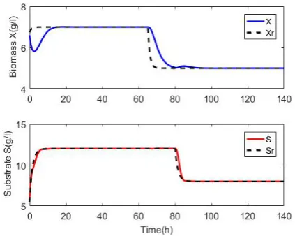
The initial conditions are x0 = (6.6 5.50)T and the

obtained results are shown in Figures 1 and 2, the tra-jectory tracking is achieved, where the biomass and the substrate concentrations follow the desired outputs. In addition, the constraints on the inputs controlD(t) and

Sin(t) are respected.

Figure 1: Evolution of the system outputs

Figure 2: Control inputsD(t) andSin(t)

6.1.2 LQI control

Solving the LMIs established in (19), (20) and (21) the obtained weighting matrices are:

R=

"

0.328 0.000 0.000 0.328

#

.10−3

Q=

           

0.2529 0.0025 −₀_.₀₂₆₄ −₀_.₀₀₀₇

0.0025 0.2252 −₀_.₀₀₀₄ −₀_.₀₄₂₂ −₀_.₀₂₆₄ −₀_.₀₀₀₄ ₀_.₁₃₄₅ ₀_.₀₀₁₅ −₀_.₀₀₀₇ −₀_.₀₄₂₂ ₀_.₀₀₁₅ ₀_.₁₉₆₆            

.10−3

The controller gains are:

K1=

"

0.0202 −₀_.₀₀₈₁ ₀_.₀₀₄₄ ₀_.₀₁₀₁ −₀_.₀₇₃₆ ₀_.₀₁₂₈ ₀_.₀₀₉₈ −₀_.₀₀₅₆

(6)

K2=

"

0.0010 −₀_.₀₀₉₅ ₀_.₀₀₁₀ ₀_.₀₁₀₅ −₀_.₀₃₆₈ ₀_.₀₀₅₂ ₀_.₀₁₉₅ −₀_.₀₀₃₀

#

K3=

"

0.0317 −₀_.₀₀₉₅ ₀_.₀₀₀₈ ₀_.₀₁₀₆ −₀_.₂₀₀₂ ₀_.₀₀₃₉ ₀_.₀₁₆₅ −₀_.₀₀₀₄

#

K4=

"

0.0016 −₀_.₀₀₉₆ ₀_.₀₀₀₂ ₀_.₀₁₀₆ −₀_.₁₀₈₆ ₀_.₀₀₂₃ ₀_.₀₂₇₁ −₀_.₀₀₀₅

#

K5=

"

−₀_.₀₂₄₇ −₀_.₀₀₀₃ ₀_.₀₂₁₁ ₀_.₀₀₄ −₀_.₀₃₁ ₀_.₀₀₉₅ −₀_.₀₀₀₆ −₀_.₀₀₉

#

K6=

"

−₀_.₀₃₄₅ −₀_.₀₀₅₀ ₀_.₀₂₀₀ ₀_.₀₀₃₃ −₀_.₀₀₂₄ ₀_.₀₀₉₆ ₀_.₀₀₀₉ −₀_.₀₁₀₅

#

K7=

"

−₀_.₁₄₇₁ −₀_.₀₀₄₇ ₀_.₀₂₁₁ ₀_.₀₀₃₅ −₀_.₀₃₆₉ ₀_.₀₀₉₅ ₀_.₀₀₀₃ −₀_.₀₁₀₅

#

K8=

"

−₀_.₁₀₆₄ −₀_.₀₀₂₆ ₀_.₀₂₇₄ ₀_.₀₀₀₉ −₀_.₀₀₂₃ ₀_.₀₀₉₆ ₀_.₀₀₀₃ −₀_.₀₁₀₇

#

The Figures 3 and 4 show the simulation results using LQI control, where the controlled outputs variables achieve the desired outputs, also the constraints on control are respected.

The results obtained are comparable or even better than those obtained using the PDC controller.

6.2 Tracking control based on

recon-structed state feedback

In the practical case, only the substrate concentration is measured and the biomass is estimated, then the out-put matrix in (1) becomesC=h0 1i. For the initial conditions of system x0 = (4 8)T, the initial

condi-tions of observer ˆx0= (5 7)T and for a scalarα= 0.5,

the following observer gains are obtained:

L1=L3=L5=L7=

"

5.2458

−₁_.₃₂₀₂ #

L2=L4=L6=L8=

"

0.3483

−₀_.₆₄₄₀ #

Q=

       

5.655 0.000 −₀_.₀₀₀

0.000 4.4141 0.000

−₀_.₀₀ ₀_.₀₀₀ ₆_.₂₀₄₅        

P =

       

0.5985 0.0843 0.0000 0.0843 0.6103 0.0000 0.0000 0.0000 0.6103

       

6.2.1 PDC control

The resolution of the same LMIs in last case gives the following gains.

K1=

"

0.0231 −₀_.₀₀₄₃ ₀_.₀₀₆₇ −₀_.₁₂₉₄ ₀_.₀₀₅₈ −₀_.₀₀₃₇

#

K2=

"

−₀_.₀₀₅₇ −₀_.₀₀₄₄ ₀_.₀₀₆₆ −₀_.₁₀₈₂ ₀_.₀₀₅₈ −₀_.₀₀₃₃

#

K3=

"

0.0304 −₀_.₀₀₄₄ ₀_.₀₀₆₄ −₀_.₁₄₂₅ ₀_.₀₀₅₈ −₀_.₀₀₂₇

#

K4=

"

−₀_.₀₀₃₈ −₀_.₀₀₄₅ ₀_.₀₀₆₅ −₀_.₁₁₈₇ ₀_.₀₀₅₈ −₀_.₀₀₃₁

#

K5=

"

−₀_.₀₈₁₄ −₀_.₀₀₁₅ ₀_.₀₀₉₄ −₀_.₀₃₃₆ ₀_.₀₀₄₄ −₀_.₀₀₆₅

#

K6=

"

−₀_.₁₀₉₀ −₀_.₀₀₁₅ ₀_.₀₀₉₂ −₀_.₀₀₁₆ ₀_.₀₀₄₄ −₀_.₀₀₆₄

#

K7=

"

−₀_.₀₈₅₇ −₀_.₀₀₁₈ ₀_.₀₀₉₆ −₀_.₀₃₅₉ ₀_.₀₀₄₈ −₀_.₀₀₆₅

#

K8=

"

−₀_.₁₁₅₁ −₀_.₀₀₁₅ ₀_.₀₀₉₄ −₀_.₀₀₃₆ ₀_.₀₀₄₆ −₀_.₀₀₆₄

#

P =

       

0.0114 −₀_.₀₀₀₁ −₀_.₀₀₀₃ −₀_.₀₀₀₁ ₀_.₀₀₁₀ −₀_.₀₀₀₂ −₀_.₀₀₀₃ −₀_.₀₀₀₂ ₀_.₀₀₀₈

       

Q=



      

0.0114 −₀_.₀₀₀₁ −₀_.₀₀₀₃ −₀_.₀₀₀₁ ₀_.₀₀₁₀ −₀_.₀₀₀₂ −₀_.₀₀₀₃ −₀_.₀₀₀₂ ₀_.₀₀₀₈



      

(7)

system ( ˆS=S) after 4.33 hours. The Figure 6 presents the control inputsD(t) andSin(t), which respect the constraints.

6.2.2 LQI control

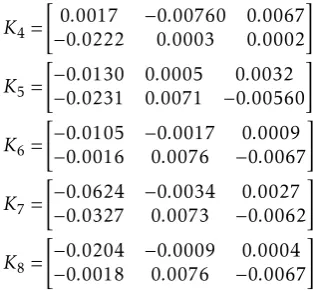
In this part, we illustrate the obtained results using LQI control. Solving the LMIs (20), (21), (19) we obtain the following controller gains and weighting matrices:

R=

"

0.2040 0.0002 0.0002 0.2028

#

.10−3

Q=

       

0.1138 0.0012 −₀_.₀₀₀₉

0.0012 0.1360 −₀_.₀₁₉₆ −₀_.₀₀₀₉ −₀_.₀₁₉₆ ₀_.₁₀₇₂

       

.10−3

K1=

"

0.0000 −₀_.₀₀₄₃ ₀_.₀₀₆₆ −₀_.₀₅₆₆ ₀_.₀₀₈₇ −₀_.₀₀₃₅

#

K2=

"

0.0015 −₀_.₀₀₇₆ ₀_.₀₀₆₇ −₀_.₀₁₂₄ ₀_.₀₀₁₅ −₀_.₀₀₀₁

#

K3=

"

0.0182 −₀_.₀₀₇₂ ₀_.₀₀₆₉ −₀_.₁₃₀₈ ₀_.₀₀₃₂ −₀_.₀₀₀₃

#

K4=

"

0.0017 −₀_.₀₀₇₆₀ ₀_.₀₀₆₇ −₀_.₀₂₂₂ ₀_.₀₀₀₃ ₀_.₀₀₀₂ #

K5=

"

−₀_.₀₁₃₀ ₀_.₀₀₀₅ ₀_.₀₀₃₂ −₀_.₀₂₃₁ ₀_.₀₀₇₁ −₀_.₀₀₅₆₀

#

K6=

"

−₀_.₀₁₀₅ −₀_.₀₀₁₇ ₀_.₀₀₀₉ −₀_.₀₀₁₆ ₀_.₀₀₇₆ −₀_.₀₀₆₇

#

K7=

"

−₀_.₀₆₂₄ −₀_.₀₀₃₄ ₀_.₀₀₂₇ −₀_.₀₃₂₇ ₀_.₀₀₇₃ −₀_.₀₀₆₂

#

K8=

"

−₀_.₀₂₀₄ −₀_.₀₀₀₉ ₀_.₀₀₀₄ −₀_.₀₀₁₈ ₀_.₀₀₇₆ −₀_.₀₀₆₇

#

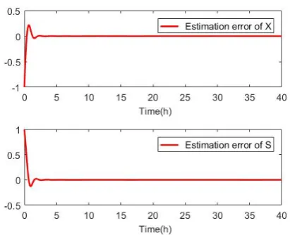
The Figures 7 and 8 present the same variables in the Figures 5 and 6 using the LQI control. where the ob-tained results indicate clearly that the desired perfor-mances can be achieved more better than the results obtained by PDC control, the Figure 9 shows the state estimation error of the state variables ( biomass and substrate concentrations), where this error tends to zero after 4.33 hours.

(8)

Figure 9: The sate estimation error

6.3 Comparison of both controllers

The outputs behaviors in the Figures 1, 3, 5, 7, show that the PDC controller presents some overshoot com-pared with LQI controller, where the PDC control re-quires the stabilization of all the different sub-models cross terms (hi(z),hj(z)) too, which increases the LMIs need to be solved. Moreover, in terms of speed, the comparison shows clearly that the LQI controller is fast than PDC one. In general, the comparison shows that the LQI controller presents the best performance.

6.4 Comparison with other methods

Another method of bioprocess control based on neural network model has been developed in [13], where the process is controlled via a neural predictive controller in that case the controller doesn’t refer to a mathemat-ical model for the process but consider the black box identification. In our case we are based on the mathe-matical model for the synthesis of the controller, the obtained results are satisfactory regarding the result obtained in [13]. Another work in the same spirit devel-oped by A. Nikfetrat [14], where the study considers a predictive controller applied to a biological feed-batch process without taking into account the constraints on the input variables and shows an important error in tracking reference trajectories, where the present work gave better results.

7 Conclusion

In this paper, the modeling and the control of the biomass growth process are treated. The objective is to control and compare two controllers. The nonlinear model of this process obtained from the mass-balance is transformed to Takagi-Sugeno fuzzy model, which represents exactly the original nonlinear model. Then, a T-S observer is designed to reconstruct the unable state when the premise variunables are not measur-able. To ensure the trajectory tracking two controllers

are tested. The PDC and the linear quadratic control. The obtained results show that the two controllers are both effective. Finds that the second controller is more stable. In addition, the inputs respect the physical con-straints of the process.

In this study, we only focus on the bioprocess control in faulty free case, that is why one interesting future work is to build a fault-tolerant control for this process.

Appendix

The proof of the Theorem 3 is presented here, we con-sider the following state estimation error:

e(t) =x(t)−_x_ˆ₍_t₎ ₍₃₄₎

their dynamic becomes:

˙

e(t) = ˙x(t)−_x˙ˆ₍_t₎

we take:

M₍_x,_{x, u}_ˆ _{) = (} r

X

i=1

hi(z)− r

X

i=1

hi( ˆz))(Aix+Biu(t)) (35)

the error dynamic then becomes:

˙

e= r

X

i=1

hi( ˆz)(Ai−LiC)e(t)+M(x,x, uˆ ) (36)

if we assume that the termM₍_x,_{x, u}_ˆ _{) satisfies the}

con-dition of Lipschitz as follows:

kM₍_x,_{x, u}_ˆ ₎k ≤_αk_x−_x_ˆk ₍₃₇₎

to ensure the convergence of (36) , one can consider the following candidate quadratic Lyapunov function:

V(e(t)) =e(t)TP e(t) (38)

leads to:

˙

V(e(t)) =Pr

i=1

hi( ˆz)e(t)T((Ai−LiC)TP+P(Ai−LiC))+ M₍_x,_{x, u}_ˆ ₎T_{P e}₍_t_{) +}_e₍_t₎T_P M₍_x,_{x, u}_ˆ ₎

(39)

Lemma 1 For two real matrices X and Y of appropriate dimensions, the following inequality is verified:

XTY+XYT < XTΩ−1X+YΩYT,Ω>0

Applying the previews lemma to the term:

M₍_x,_{x, u}_ˆ ₎T_{P e}₍_t_{) +}_e₍_t₎T_P M₍_x,_{x, u}_ˆ _{) , the derivative of}

(39) is expressed as:

˙

V(e(t))≤_eT₍_AT

i P−CTLTi P +P Ai−P LiC+α2I+P P)e (40) If there exists a symmetric and positive definite matrix

Q=QT such that:

AT_i P−_CT_LT

(9)

leads to:

−_Q₊_α2I+P P <0 (42) Finally, we apply the Schur complement to (42) we obtain:

"

Q−_α2I P

P I

#

>0 (43)

Then the proof is completed.

References

[1] V. Vastemans, M. Rooman, P. Bogaerts, “A robust method for the joint estimation of yield coeffcients and kinetic parameters in bioprocess models”, Biotechnology Progress 25 (3), 2009, 606–618. doi:10.1002/btpr.89.

[2] A. Karama, O. Bernard, J.-L. Gouz´e,“ Constrained Hybrid Neu-ral Mod- elling of Biotechnological Processes”, International Journal of Chemical Re- 70 actor Engineering 8 (1), 2010, 1–15. doi:https://doi.org/10.2202/ 1542-6580.2117.

[3] V. Grisales, A. Gauthier, G. Roux, “Fuzzy Optimal Control Design for Dis- crete Affine Takagi-Sugeno Fuzzy Models: Application to a Biotechnologi- cal Process”, 2006 IEEE In-ternational Conference on Fuzzy Systems, 2006, 2369–2376, doi:10.1109/FUZZY.2006.1682030.

[4] E. Herrera, B. Castillo, J. Ramrez, E. C. Ferreira, “Takagi-sugeno multiple- model controller for a continuous bak-ing yeast fermentation process”, ICINCO 2007 - 4th In-ternational Conference on Informatics in Control, Au-tomation and Robotics, Proceedings ICSO, 2007, 436–439. doi:10.5220/0001622704360439.

[5] Min-Sen Chiu, Shan Cui, Qing-Guo Wang. “ Internal Model Control Design for Transition Control”, AIChE journal, vol 46, 2000

[6] E. J. Herrera-Liopez, B. Castillo-Toledo, R. Femat, “Fuzzy servo controller 65 for CSTB with substrate inhibition ki-netics”, Journal of Process Control 22 (6) (2012) 959–967. doi:10.1016/j.jprocont.2012.05.003.

[7] A. M. Nagy Kiss, B. Marx, G. Mourot, G. Schutz, J. Ragot, “Observers design for uncertain Takagi-Sugeno systems with unmeasurable premise variables and unknown inputs. Appli-cation to a wastewater treatment plant”, 30 Journal of Pro-cess Control 21 (7), 2011, 1105–1114. doi:10.1016/j. jpro-cont.2011.05.001.

[8] M. Bouharkat, M. Ramdani,“ Fuzzy observer based pre-dictive control of an activated sludge depollution biopro-cess”, 2013 International Conference on Control, Deci-sion and Information Technologies, CoDIT, 2013, 236–241. doi:10.1109/CoDIT.2013.6689550.

[9] E. Herrera, B. Castilloa, J. Ramrezb, E. C. Ferreirac, “Exact fuzzy observer for a baker’s yeast fermentation process”, IFAC Proceedings Volumes (IFAC- PapersOnline) 10 (1), 2007, 313– 318. doi:10.1109/FUZZY.2007.4295502.

[10] S. Aouaouda, M. Chadli, M. T. Khadir, T. Bouarar, “Ro-bust fault tolerant tracking controller design for un-known inputs T-S models with unmeasurable premise vari-ables”, Journal of Process Control 22 (5), 2012, 861–872. doi:10.1016/j.jprocont.2012.02.016.

[11] S. Bououden, M. Chadli, H. R. Karimi, “Control of uncer-tain highly nonlinear biological process based on Takagi-Sugeno fuzzy models”, Signal Processing 108 (2015) 195–205. doi:10.1016/j.sigpro.2014.09.011.

[12] S. Carlos-Hernandez, E. N. Sanchez, J. F. B´eteau, “Fuzzy ob-servers for anaerobic WWTP: Development and implemen-tation”, Control Engineering Practice 17 (6), 2009, 690–702. doi:10.1016/j.conengprac.2008.11. 008.

[13] A. Karama, “Contribution à la modélisation et la commande par réseaux de neurones des bioprocédès”, thesis, University Cadi Ayyad, Faculty of Science Semlalia Marrakech, 2004.

[14] A. Nikfetrat, A.R. Vali, V. Babaeipour. “Neural Network Mod-eling and Nonlinear Predictive Control of a Biotechnological Fed-batch Process”, IEEE International Conference on Control and Automation Christchurch, New Zealand, December 9–11, 2009.

[15] Mohd N, Aziz N. “Performance and Robustness Evaluation of Nonlinear Autoregressive with Exogenous Input Model Predic-tive Control in Controlling Industrial Fermentation Process”, Journal of Cleaner Production, 2016.

[16] O. Gehan, E. Pigeon, M. Pouliquen, L. Fall, R. Mosrati, “Non-linear control of dissolved oxygen level for Pseudomonas putida bacterium fermentation”, 15 2016 IEEE Conference on Control Applications, CCA 2016 (2016) 1215– 1220 doi:10.1109/CCA.2016.7587972.

[17] K. Tanaka, H. O. Wang, “Fuzzy Control Systems Design and Analysis”, John Wiley and Sons, Inc., New York, USA, 2001. doi:10.1002/0471224596.

[18] Saifia, D., Chadli, M., Labiod, S., and Guerra, T. M., “ Robust H∞_{Static Output Feedback Stabilization of T-S Fuzzy Systems} Subject to Actuator Saturation”, Int. J. Control Autom. Syst. 10(3), 613–622, 2012

[19] Hassan.K.Khali. “Nonlinear Systems”, second edition, Prentice Hall. United States of America, 1996.

[20] Guechi, El-Hadi, Lauber, Jimmy, Dambrine, Michel, et al., “PDC control design for non-holonomic wheeled mobile robots with delayed outputs”, J. Intell. Robot. Syst. 60(3-4), 395–414, 2010

[21] Xu, Bin, Wang, Shixing, Gao, Daoxiang, et al., “Command fil-ter based robust nonlinear control of hypersonic aircraft with magnitude constraints on states and actuators”, J. Intell. Robot. Syst. 73(1-4), 233–247, 2014

[22] Zhu, Senqiang et Wang, Danwei., “ Adversarial ground target tracking using UAVs with input constraints”, J. Intell. Robot. Syst. 65(1-4), 521-532, 2012

[23] M. Abyad, A. Karama, A. Khalloq, “Fuzzy Takagi-Sugeno Based Modelling and Control For an Alcoholic Fermentation Process”, 3rd International Conference on Electrical and Information Technologies ICEIT, Rabat, Morocco, 2017.

[24] P. Bergsten, R. Palm, D. Driankov, “Fuzzy observers”, 10th IEEE International Conference on Fuzzy Systems. (Cat. No.01CH37297) 2, 2001, doi:10.1109/FUZZ.2001.1009051.