Wavelet denoising for postprocessing of a 2D Particle - In - Cell code

February 2007, Vol.16, 195-210 Eric Canc`es & Jean-Fr´ed´eric Gerbeau, Editors

DOI: 10.1051/proc:2007013

WAVELET DENOISING FOR POSTPROCESSING OF A 2D

PARTICLE - IN - CELL CODE

Salimou Gassama

, ´

Eric Sonnendr¨

ucker

, Kai Schneider

, Marie Farge

and

Margarete O. Domingues

Abstract. In this paper, we aim at improving the accuracy of a Vlasov-Poisson solver using a 2D Particle-In-Cell (PIC) scheme, by denoising its charge density field. To this end, we have used an improvement of Donoho and Johnstone’s wavelet denoising technique. To some extent, our work is a continuation of that performed by Chehab et al.[6]. Indeed, they made such a study in the one dimensional case and validated their analysis by considering the simulation of the Landau damping phenomenon. They concluded on the efficiency of the method in reducing the number of particles. However, our approach is quite different, since we do not use wavelets to directly interpolate the charge density, but we smooth the density field calculated by the PIC code. This is carried out via an iterative wavelet denoising technique introduced by Azzaliniet al.[2]. Our work consists in studying the application of the method as a post-processing tool, in view of a future embedding into the PIC code. The results are the following: first, we showed that the hypotheses underlying the application of this method are valid. Secondly, we can infer from this study that it is possible to significantly reduce the amount of data needed for a simulation.

R´esum´e. L’objectif de ces travaux est d’accroˆıtre la pr´ecision d’un solveur Vlasov-Poisson bas´e sur un sch´ema de type Particle-In-Cell (PIC). Pour ce faire, `a l’instar de Chehab et coll. [6], nous avons choisi d’utiliser des techniques d’analyse multir´esolution par ondelettes pour d´ebruiter la densit´e de charge. Cependant, `a la diff´erence de ces auteurs, nous effectuons un post-traitement de la densit´e de charge en appliquant une technique it´erative mise au point par Azzalini et coll. [2]. Cette ´etude est un pr´ealable `a l’impl´ementation d’un algorithme de d´ebruitage dynamique du code PIC. Les exp´eriences num´eriques men´ee sur le cas-test de l’amortissement Landau nous ont permi de valider les hypoth`eses sous-jacentes et portent `a croire qu’il est possible de r´eduire de mani`ere significative le nombre de particules n´ecessaires pour une pr´ecision donn´ee.

∗_CIRM

∗∗_{CEMRACS 2005} ∗∗∗_CNRS

∗∗∗∗_{DFG (Graduiertenkolleg 366)}

1_{Institut de Recherche Math´ematique Avanc´ee, UMR CNRS 7501 Universit´e Louis Pasteur, Strasbourg, France} 2_{MSNM–CNRS & CMI, Universit´e de Provence, 39 rue Joliot–Curie, 13453 Marseille cedex 13, France}

3_{LMD–CNRS, Ecole Normale Sup´erieure, 24 rue Lhomond,75231 Paris cedex 05, France}

4_{Laborat´orio Associado de Computa¸c˜ao e Matem´atica Aplicada (LAC), Instituto Nacional de Pesquisas Espaciais (INPE), Av.}

dos Astronautas, 1758, 12227-010 S˜ao Jos´e dos Campos, Brasil

c

EDP Sciences, SMAI 2007

Introduction

We shall first recall the physical background of the problem at hand, as well as its mathematical modeling. Given the main purpose of this report, we will only point out the aspects which are useful to seize the core of the matter discussed in this paper. For a thorough insight into it, one could refer to e.g.: [5, 16, 17, 20] and the bibliographies therein. Though notations will be introduced as we encounter new expressions, it is convenient to note that from now on, all magnitudes denoted with a subscripte, i, orM, will respectively refer to those relative to electronic, ionic and model magnitudes.

As far as we are concerned, we will consider the kinetic model of plasmas of charged particles in which the collisions between particles are neglected. Moreover, due to the fact that we consider a non relativistic plasma in a quasi-stationary regime we will neglect the magnetic field. Thus the Vlasov-Poisson equation for a single particle species of chargeqand massmreads as follows:

∂f

∂t +v· ∇xf −q·(E· ∇p)f = 0, (x, v)∈R

d_×Rd_{, (0.1)}

where f(x, p, t) is the particle the distribution function with respect to position x, momentum p = mv and time t. E is the electrostatic field. This equation models the invariance of the distribution function f along the trajectories of the particles moving through the electrostatic field. The self-consistent field produced by the charge of particles is:

Eself(x, t) =−∇xφself(x, t) with

−Δxφself = ρ(x, t)

ρ(x, t) = q f(x, p, t) dp (0.2)

In order to confine the particles in a bounded domain, we consider the classical case of an additional external potential φext(x), which can be generated e.g. by a constant background of ions such that:

E(x, t) =E_self+E_ext≡ −(∇_xφ_self+∇_xφ_ext) (0.3)

To close the systems to be dealt with, we shall also fix an initial distribution function, via:

f(x, p,0) =f0(x, p) (0.4)

Particle simulations [5,17] try to mimic this behavior at best. In this study, we use Particle-In-Cell (PIC) meth-ods. PIC methods consist in modeling the medium as a finite set of individual elements (particles) interacting with one another. However, if we also assume (see [5]) that the Debye length is invariant, that is: λ_D,M =λ_D, then the model and real plasma temperatures will be different: T_e,M = αT_e, though the thermal velocities remain the same:

v_T,M =

Te,M m

₁/2

=v_T (0.5)

Consequently, the mean free path in a PIC plasma is much smaller than that of a real plasma. As a consequence, the level of shot noise is much higher in the model plasma. A means of reducing this effect could consist in increasing the number of particles per cell in the Eulerian mesh. However, it proves to be highly computationally expensive.

Thus in this paper, we try to control the noise intrinsically generated by the model. More precisely, we aim at enhancing accuracy, meanwhile significantly reducing the number of particles per cell. That is why we used the optimal compression abilities of wavelets [10–12, 21], in order to have such an adaptive code. To meet these requirements, we passively denoised the PIC code via an ad-hoc postprocessing tool. This is a preliminary step before a future embedding of the procedure into the PIC code.

and 4 are respectively devoted to the presentation and discussion of the application of these techniques to the classical Landau damping.

1.

Plasma modeling via Particle–In–Cell methods

Now, we focus on the numerical schemes used to model the aforementioned physical problem. For a compre-hensive presentation, the reader may refer to [3].

First and foremost, the initial distribution functionf_N0(x, p), of a species is approximated via a linear com-bination of N Dirac mass tensor products associated to macro-particles with initial states (x0_k, p0_k) in phase space:

f_N0(x, p) = N

k=1

wkδ(x−x0k)δ(p−p0k) (1.6)

Besides, we draw the reader’s attention to the fact that the choice of plasma particle initial distribution in phase space coordinates is of great importance in discrete models, since it affects the possibility of an adequate investigation of the physical processes considered. Here, we use a Monte Carlo method called ”quietstart” (see e.g. [17] for more details on statistical PIC methods). Then, each time step of the simulation is split into two phases:

During the first stage , the interactions or the result of the joint effect of particles with fixed state are calculated. This is done by solving the Poisson equation 0.2. To solve the Poisson equation, we use the Fourier transform method. For the Vlasov equation, we solve it by considering its characteristic curves:

⎧ ⎨ ⎩

dX(t)

dt = V(t)

dV(t)

dt =

q

mE(X(t), t)

(1.7)

This is the most difficult task, since we have to deal with a nonlinear coupling. The electric field known at the nodes of the Eulerian grid are interpolated to the positions (in phase space) of the particles. To interpolate this magnitude, we use shape functions {Si} associated to the Eulerian nodes{xi}. If we denote byVi the volume of the cell associated to nodexi, then we shall impose

V_iS_i(x) = 1 ∀x∈R2to ensure charge conservation. Concerning the spline functions, we recall that a spline of order m can be obtained from the 0–order spline 1|_[−1/2,1/2] viam convolutions of the latter by itself. The electric field is interpolated as being:

E(xk(t)) =Vk

i

E(xi, t)Si(xk(t)) (1.8)

During the second stage, by using a leapfrog scheme, we can advance particles in two steps according to the Newton law for momentum: _⎧

⎪ ⎨ ⎪ ⎩

v_kn+1/2−vn_k−1/2

Δt =

q mEkn

xn+1_k −xnk

Δt = v

n+1/2 k

(1.9)

Therefore, we have to calculate the new charge density{ρh(xi, t)} at the nodes of the Eulerian grid. This is the second interpolation and is carried out by using the same shape functions as above, in order to avoid the apparition of self-forces [18]:

ρN(x, t) = q

R2fN(x, p, t) dp = qN_k=1wkδ(x−xk(t)) ρh(xi, t) =

R2ρN(x, t)Si(x) dx = qN_k=1wkSi(xk(t))

Finally, knowing the charge density, we can compute the electric field for the next time step. Let us recall the fact that all the difficulty lies in the interpolation between Lagrangian and Eulerian meshes. Indeed, it may lead to charge non conservation. To solve this problem, several solutions have been suggested, such as constraints via Lagrange multipliers (see [3]). However, for the general Vlasov-Maxwell equations, methods calculating the current such that charge conservation is satisfied are noisier. To reduce numerical noise, one can use higher order shape forms. In the next section, we will introduce another technique to reduce that noise: wavelet filtering.

2.

Wavelet denoising of a 2D PIC code: technical aspects

2.1.

Basics on wavelet theory

In what follows, we will recall some basic assumptions on wavelets, so that the paper is self-contained. Besides, we will only consider the case of discrete wavelet transforms. For further readings, we refer to [7, 9, 23]. In a nutshell, the wavelet transform decomposes the original data into a coarse approximation and a sequence of finer and finer details, keeping the size of the data constant. In this respect the wavelet transform has adaptive time/space frequency resolution. Moreover, it is also faster1than the Fast Fourier Transform. The framework of this approach is laid on a special construction of orthonormal bases ofLp_{(R) with 1< p <∞generally taken} to be equal to 2. Such a basis is obtained thanks to a couple (ϕ , ψ) of functions respectively called thescaling and thewavelet function. These bases are defined by an iterative algorithm of dilatation and translation of the functionsϕandψ. Such a procedure has led to the concept called multiresolution analysis (MRA). MRA gives rise to the multiscale local analysis of the signal and fast numerical algorithms. To give more details about this procedure, let us first recall the following definitions:

Definition 2.1. Riesz2 basis of a Hilbert space: Let (uk)k∈Zbe a sequence of a Hilbert space. It is then called

a Riesz basis, if there exists two strictly positive constantsAandB such that, for any finite sequence (xk)k∈I⊂Z

we have:

Ax₂≤ (u_kx_k)_k∈Z2≤Bx₂ (2.11)

Definition 2.2. Multiresolution analysis ofR: it consists of a functionϕ∈L2(R) of unit norm and an increas-ing sequence{Vj}_j∈Z of closed linear subspaces ofL2(R) defined by: Vj =span

{ϕj,k≡2j/2ϕ(2j · −k)}k∈Z

, with the following properties:

(1) The family (ϕ₀,k)k∈Z is a Riesz basis

(2) _j∈ZVj={0}

(3) _j∈ZVj is dense inL2(R) (4) (∀j∈Z)(V_j ⊂V_j+1)

We will also consider the following orthogonality hypothesis: (5) (∀j, k, l∈Z)(ϕ_j,k, ϕ_j,l=δ_k,l)

Remark 2.3. From the definition of a Riesz basis, we may infer from the first and the fourth statements of this definition, that there exists a sequence – called thelow-pass filter – (h_k)_k∈I⊂Zof finite3support, such that:

ϕ(·) =√2 k∈Z

h_kϕ(2 · −k) (2.12)

This equation is calledrefinement equation.

To construct orthogonal wavelets, letW₀ be the orthogonal complement of V₀ in V₁, that is: V₁ =V₀⊕W₀. Then there exists a function, called themother of waveletsψsuch that (ψ₀,k≡ψ(· −k))k∈Z is an orthonormal

1_{O(NlogN) versusO(N),N being a characteristic size of the system}

2_{So far, the most general context for wavelet design lies on the notion offrames, but for the sake of concision and because it is} sufficient, we will only refer to Riesz bases.

basis ofW₀. Accordingly, (ψ_j,k≡2j/2_ψ(2j _{· −k))}

j,k∈Zis an orthonormal basis of ofWj, whereVj+1=Vj⊕Wj. Similarly to the case ofϕ, fromψ∈W₀⊂V₁, we have another filter – thehigh-pass filter – (g_k)_k∈Z such that:

ψ(·) =√2 k∈Z

gkϕ(2 · −k) (2.13)

If the low-pass filter h has D non-vanishing coefficients, then a permissible choice for g is : (∀k ∈ Z)(gk = (−1)k_h

D−k−1). Given this setting, we can decompose any function ofL2(R) via its projections on these spaces. LetPj andQj be respectively the orthogonal projections on spacesVj andWj. Then we have:

(∀f ∈L2(R))(Pj+1f =Pjf+Qjf) (2.14)

With:

Pjf =

k∈Zf, ϕj,kϕj,k Qjf =

k∈Zf, ψj,kψj,k (2.15) Consequently, we have these two decompositions ofL2(R):

L2(R) =⊕jWj =Vj0⊕ ⊕j≥j0Wj (2.16)

Then, the means to apply a discrete wavelet transform will only consist in performing a change of basis trans-formation between the bases ofVj+1 and Vj⊕Wj. By using respectively 2.12 and 2.13, in the expressions of ϕj,k andψj,k, we are led to:

ϕj,k =

D+2k−1

l=2k hl−2kϕj+1,l ψj,k =

D+2k−1

l=2k gl−2kψj+1,l

(2.17)

From which we deduce the following decomposition algorithm connecting coefficients of successive approxima-tions:

(∀f ∈L2(R))

cj,k≡ f, ϕj,k =

_D+2k−1

l=2k hl−2kcj+1,l dj,k≡ f, ψj,k =

_D+2k−1

l=2k gl−2kdj+1,l

(2.18)

Finally, thanks to 2.17, 2.14 and the orthogonality property, we obtain the reconstruction formula:

cj+1,k= D−1

l=0

hk−2lcj,l+ D−1

l=0

gk−2ldj,l (2.19)

Last but not least, for practical reasons, one has to consider a finite subset of integers for the scale indexj. So, letJc < Jf be the chosen coarsest and finest resolution levels, the applying 2.18 recursively yields:

VJf =VJc⊕

Jf−1

j=Jc Wj (2.20)

Thus, we have:

f ≈ D−1

k=0

f, ϕ_Jf,kϕ_Jf,k= D−1

k=0

f, ϕ_Jc,kϕ_Jc,k+ Jf−1

j=Jc

D−1

k=0

f, ψ_j,kψ_j,k (2.21)

Remark 2.4. A means to make a multidimensional wavelet analysis of data consists in building tensor product spaces of the spaces{V_j}_j∈Z. In dimension two, we have:

∀j∈Z, Vj+1 = Vj+1⊗Vj+1 (2.22)

= (Vj⊗Vj)⊕(Wj⊗Vj)⊕(Vj⊗Wj)⊕(Wj⊗Wj) (2.23)

a practical point of view, if we have to handle a square matrix, then we perform a 1D wavelet transform on each column and line for a given resolution level.

At this stage, it necessary to recall that nowadays, there is a whole range of wavelet families available. Hence the necessity of knowing how to choose those which would best meet the requirements of the application at hands. These requirements may concern e.g. time/space localization, frequency localization, the speed of the transform, or the compression/reconstruction abilities. In our case, the latter aspect is of first importance. However, all these properties are interrelated. To obtain such and such property, one has to analyse the following characteristics:

• The size of the support of the wavelet function. • The symmetry of the wavelet function.

• The number of vanishing moments4.

• The regularity of the wavelet and scaling functions. • The orthogonality of the basis.

For the problem at hands, we should bear in mind that compression is all the more better than the wavelets have a large number of vanishing moments. However, due to the errors introduced by the thresholding process, we will need wavelets with high regularity in order to enhance the quality of the reconstructed data. Moreover, since we assume the additive noise to be well modeled by independent and identically distributed Gaussian vari-ables, the transform should preserve the independence property. Yet, this can granted by the use of orthonormal wavelets (see [23]).

Among the wavelets that meet the above stated requirements, are the classical Daubechies orthonormal wavelets with compact support. Actually, it can be proved that a Daubechies wavelet withrvanishing moments hasμr(μ≈0.2) continuous derivatives. However, we should be aware of the fact that as regularity increases, so does the support. Now, a small support is needed for a faster transform, while it implies relatively few vanishing moments and low regularity. This means that the requirements above cannot be satisfied equally well. Indeed, the size of the support, the symmetry of the wavelet function affect time/space localization, while the number of vanishing moments and the regularity affect the frequency localization. Good time/space localization requires a small support and high symmetry, while good frequency localization requires many vanishing moments and high regularity. A small support is also needed for a faster transform. However, a small support implies relatively few vanishing moments and low regularity. In addition, orthogonality implies asymmetry, except for the simplest wavelet (the Haar wavelets). (Bi-)orthogonality5weakens the coupling between the properties of the decomposition and reconstruction wavelets, and allows perfect symmetry. In order to fulfill the requirements of the problem at hands we decided to choose a wavelet family called ’Coiflets’, which has the advantage that both the scaling and the wavelet function have vanishing moments.

2.2.

Wavelet denoising techniques

In this section, we shall detail the nonlinear wavelet denoising techniques that we used to denoise the charge density field. Our purpose is to significantly reduce the number of particles needed to perform the simulation described in section 2. Indeed, due to the numerical noise, so far good accuracy can be obtained only with a large number of particles. To denoise our 2D PIC code, we use the most important abilities of wavelets: multiresolution and compression. Actually, the wavelet transform cuts up the signal into different frequency components and then enables us to study each component with a resolution matched to its scale. The first application to denoising was developed by D. Donoho and I. Johnstone. For further readings, we refer to [10–12, 21] for wavelet denoising theory, and [13–15, 24, 25, 27] for its application to the study of some physical processes.

4_{A waveletψ has N vanishing moments when}∞

−∞xkψ(x)dx= 0, for 0≤k≤N−1. Wherexdenotes time or space. In

particular, all ”normal” wavelets have zero mean (i.e. N ≥ 1), since under rather general assumptions, this is related to the admissibility condition for the existence of the inverse transform.

Let us assume that we wish to estimate the signals, which is corrupted with additive Gaussian white noise, i.e. we observe:

f =s+w (2.24)

Wherew∈ N(0, σ) is a Gaussian white noise with varianceσ. Then, if we denote by ˇs an estimator of s, we define arisk associated to this estimation by the following:

Definition 2.5. Letκbe a convex even function, called thecost. Then the therisk Rassociated to this cost is defined by:

R(ˇs, s) =Es[κ(ˇs(f)−s)] (2.25)

For a large class of cost functions, simply choosing the estimator ˇsequal to the valuef leads to minimizing the risk operator:

R(f, s) = inf ˇ

s sup_s R(ˇs, s) (2.26)

Whence the calling minimax, since we have the best estimation in the worse case. If we have to handle an evolution problem, that is s varies with the time variable, then the problem at hands becomes trickier. However, in this case, the knowledge of some a priori information about the regularity ofsmay enable us to find its best estimator. LetE be a known regularity space to whichsbelongs. Then the estimator should be the solution of:

inf ˇ s _ssup

E≤C

R(ˇs, s) (2.27)

Despite estimators have been found for several functional spaces, such an approach is limited at least due to two obstacles. First, from a computational point of view, the convergence rate of those algorithms depends on the functional space. Secondly, the unknown function may simultaneously belong to several functional spaces, or worse: we often do not have any clue about its regularity (e.g.: a noisy image). It is in this context that Donoho and Johnstone introduced new methods based on wavelet decomposition. Indeed, thanks to the unconditionality6property of wavelet bases, such methods allow us to have convergence rates of the same order of magnitude on a whole set of functional spaces. The payback is then a not exactly – though near to – minimax risk. The first method – calledWavelet shrinkage– introduced by these authors in [11] and consists in replacing the wavelet coefficients{d_j,k}_j,k∈Zof the noisy function by:

sign(d_j,k) inf(|d_j,k| −,0) (2.28)

Where the threshold is fixed with respect to the known or estimated variance of the noise. In the orignal article of these authors, an optimal value of the threshold was proved to be equal to =√2σlogN, where

N corresponds to the number of grid points or the size of the sample. This value was calculated under the assumption that the observations are independent identically distributed random variables withN(0, σ) density. This method is as efficient as the minimax estimator in many functional spaces and minimizes the maximum

L2-risk – i.e.: κ ≡ · 2₂ – in a whole class of finite energy signals including H¨older and Besov spaces. In addition, in the worse case, the risk estimation error is approximatively logN.

In this paper, we used an improvement of this method suggested by [2], in which the estimation of the variance is made via an iterative algorithm performed on the threshold residuals. More precisely, the following algorithm is applied:

(1) Initialisation

- Apply a fast wavelet transform to the initial data {si}_1≤i≤N to obtain the wavelet coefficients {ˇsi}_1≤i≤N.

- Compute the variance_√ σ₀ of these coefficients and set the initial threshold to be equal to t₀ = 2σ₀logN.

- Set the noise counter variableν_Noise to be equal toN. (2) Main loop

At each stepi, repeat:

- Setν_Noise =ν_Noiseand setν_Noiseto be the number of coefficients such that their modulus is smaller thanti.

- Compute the variance σi+1 from the wavelet coefficients inferior to ti and set the new threshold ti+1 to the value

2σi+1logN. - Increment the counteri. Untilν_Noise =νNoise.

(3) Final step

- Use the inverse fast wavelet transform to compute the denoised data from the coefficients such that their absolute value is greater than the last threshold value.

3.

Application to passive denoising of a PIC code: numerical results

3.1.

The Landau damping case test

Here, we shall discuss the results obtained from these numerical experiments and sketch some perspectives for future extensions of the method. The Landau damping test is known for its efficiency to assess the quality of Vlasov–Poisson or Vlasov–Maxwell codes. For the sake of clarity, let us briefly recall the physical background related to it.

In stable plasmas electrostatic waves are damped due to wave–particle interactions, and not to collisions. This is the meaning of the Landau damping. Indeed, letωdenote frequency andkthe wave vector. Then let us consider particles with velocities just larger than the wave phase velocityuω/k. They can gain or lose energy depending on the relative phase of the wave; but if they gain energy, their velocity increases and they go out of the resonance: they can not exchange energy any more. If they lose energy, they slow down and stay longer in the resonance. So overall, they transfer energy to the wave. The opposite holds for particles with velocities just below the phase velocityuω/k. Those that gained energy from the wave remain in the resonance longer, and the net effect is that they gain energy from the wave. The total energy balance is therefore given by the ratio between how many particles gain energy from the wave (withuω/k and how many give energy to the wave (uω/k). This balance can be deduced from the slope of the distribution functionf₀(u) around the resonance

u≈ω/k. This is the meaning of the formula:

γ∝ df0 du

u=ω/k

(3.29)

i.e. the damping is proportional to the slope of the equilibrium distribution function at the wave phase velocity (the wave–particle resonance).

For our numerical experiments, we consider a configuration with periodic boundary conditions and the initial distribution function is chosen so as to be a perturbed Maxwellian:

f0(x, v) = √n0 2πvT

exp

−vx2+vy2 2v2_T

(1 +αcos(kxx)) (3.30)

The phase space domain is denoted by Ω≡[0, L_x]×[0, L_y]×R2. Besides, perturbation amplitudeα, the thermal velocity vT, as well as the x–component kx of the wave vector are constant. Consequently, this perturbation of period Lx = 2_kπ_x creates a perturbed electric field such that the norm of its kx-th mode decays with an exponential rate according to the law:

where under the conditionk_x2λ2_D 1, we have:

γ≈ −

π

8

ω_e

(kxλD)3 exp

− 1

2(kλD)2 − 3 2

(3.32)

ω ≈ω_e1 + 3(k_xλ_D)2 (3.33) In order to diminish numerical roundoff errors caused by huge or tiny magnitudes, the PIC code used here was implemented by considering dimensionless Vlasov–Poisson and Maxwell equations. To this end, we make the following changes of variable in equations 0.1 to 0.4:

t= ¯tt, x= ¯xx, v= ¯vv, E= ¯EE,

ρ = ¯ρρ, q =qeq, m=mem, (3.34)

whereme= 9.109410−31kg is the electron mass, and variables with a prime symbol are those expressed in the SI unit system. Those with a bar represent the new units. This leads us to the following dimensionless Vlasov equation:

∂f ∂t +

¯

v¯t

¯

xv· ∇xf+

¯

xtqω¯ _e2

¯

vm E· ∇vf = 0 (3.35)

In order to fix the units of the variables, we state that:

¯

t=ω−_e1, ¯v=v_T =c/8, x¯= ¯vt¯ ¯

w= ¯fx¯2¯v2=n₀¯x2, ρ¯=q_en₀, E¯ =x¯ρ¯

0

(3.36)

Wherec is the speed of light and ¯wis the new mass unit of macroparticles. In this new unit system, we have:

¯

v= 3.7474107m/s, ¯t= 1.772710−2n₀−1/2s, x¯= 6.6430104n−₀1/2m

¯

E= 1.202010−2n1₀/2V /m, ρ¯= 1.602110−19n₀C/m2, w¯= 4.41291011n₀

We carry out the subsequent numerical experiments with the following values for the constants:

α= 0.1, kx= 0.5, ωe= 1, λD= 1

In these conditions, the theoretical exponential decay rate of the the electrostatic field is predicted to be

γ ≈ −0.151 with an oscillation frequency of ω ≈ 1.323. As for the mesh grid, we used a uniform grid of 128×128 in (x, y)-coordinate plane. Finally, we consider this configuration with different particle densities: from 50 to 2000 particles per cell.

3.2.

Numerical results of the passive denoising

In this part of the numerical experiment, we simulated the aforementioned case test with different numbers of particles per cell (nppc): from one to 2000. We use the Coiflet filters7, which yield wavelets (and scaling functions) of length 12, which yield wavelets with 4 vanishing moments. Then, we used a postprocessing program based on the algorithm described in section 3, to denoise the resulting fields.

To assess the time evolution of the noise, we studied the variation of some image quality parameters with respect to the number of particles per cell. Namely, we observed the time trend of the compression rate (in %), the signal to noise ratio SNR (in dB) and the variance ratio of the coherent and noisy solutions (in %). Let us recall that in what is following, coherent part and denoised signal are taken for synonyms. The same applies to incoherent part and noise component. A quantitative summary of the evolution of these features is provided by table 1.

nppc Compression rate: 100NWCcoh

NWCtot (%) SNR: 10 log(

RMS

RMSinc) (dB) 100

RMScoh

RMStot (%)

50 0.06 2.5 44.4

500 0.02 11.0 92.0

1000 0.15 14.8 96.7

1500 0.15 16.7 97.9

2000 0.18 18.1 98.4

Table 1. Summary of the compression rate and the SNR as a function of the nppc.

0 20 40 60 80 100 120 0

50 100 −0.2 −0.15 −0.1 −0.05 0 0.05 0.1 0.15

Noisy charge density field for 2000 ppc

X−Y plane: mesh node numbers

Z axis: charge density value

−0.1 −0.05 0 0.05 0.1

0 20 40 60 80 100 120

0 50 100 −0.1 −0.05 0 0.05 0.1

Coherent charge density field for 2000 ppc

X−Y plane: mesh node numbers

Z axis: charge density value

−0.08 −0.06 −0.04 −0.02 0 0.02 0.04 0.06 0.08

Figure 1. Surface plots of the charge density fields for 2000 ppc. Noisy PIC solution (left), denoised PIC solution (right)

Let us sum up the main deductions that can be drawn from the study of these data. We denote by NWC the number of coefficients of the wavelet decomposition, and by RMS the standard deviation of these coefficients. Subscripts ’coh’, ’inc’, and ’tot’ respectively refer to the coherent , the incoherent and the whole signal. As it was announced in the previous sections, we observe that the incoherent part of the signal becomes all the more negligible that the nppc increases (see also figures 3 and 4). As a consequence, a simulation with a high enough nppc may be taken as a reference solution for the study of accuracy features. Another information given by this table, is that we need extremely few wavelet coefficients to reconstruct the solution (less than 0.2 %). It indicates that the solution is highly regular. Finally, we see that the signal is highly blurred for low nppc, since less than half of the total energy is considered as being coherent for 50 ppc.

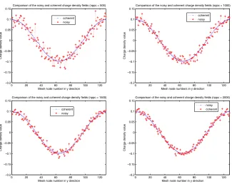
Images on figure 1 are obtained with 2000 ppc and give us an insight of the exact solution. According to table 1 and the comments we made upon it, it seems reasonable to take the case of 2000 ppc as a reference to study the influence of the number of particles on the accuracy of the reconstruction. Thanks to the symmetry of the problem (whence of the solution), we could use cuts made at the middle mesh node number 64. In a first stage, we compared our reference solution with coherent solutions obtained with different nppc (see the curves of figure 2). In the second stage, we compared all coherent solutions with their respective noisy counterparts. The results are furnished by the curves of figures 3 and 4.

0 20 40 60 80 100 120 −0.2 −0.15 −0.1 −0.05 0 0.05 0.1 0.15

Mesh node number in y direction

Charge density value

Comparison of coherent charge density fields from 1 to 2000 ppc

2000 ppc 1500 ppc 1000 ppc 500 ppc 250 ppc 100 ppc 50 ppc 25 ppc 10 ppc 5 ppc 2 ppc 1 ppc

0 20 40 60 80 100 120 −0.2 −0.15 −0.1 −0.05 0 0.05 0.1 0.15

Mesh node number in y direction

Charge density value

Comparison of the coherent charge density fields with 1 to 10 ppc versus the reference case of 2000 ppc

1 ppc 2 ppc 5 ppc 10 ppc 2000 ppc

0 20 40 60 80 100 120 −0.2 −0.15 −0.1 −0.05 0 0.05 0.1 0.15

Mesh node number in y direction

Charge density value

Comparison of the coherent charge density fields with 25 to 100 ppc versus the reference case of 2000 ppc

25 ppc 50 ppc 100 ppc 2000 ppc

0 20 40 60 80 100 120 −0.1 −0.08 −0.06 −0.04 −0.02 0 0.02 0.04 0.06 0.08 0.1

Mesh node number in y direction

Charge density value

Comparison of the coherent charge density fields with 250 to 1500 ppc versus the reference case of 2000 ppc

250 ppc 500 ppc 1000 ppc 1500 ppc 2000 ppc

Figure 2. _{Comparison of the reference coherent PIC solution with those having less particles} per cell. Cuts of the charge density field for different nppc

solution as soon as we have 250 ppc. This gives us incentives for reducing the number of particles per cell while enhancing accuracy.

Meanwhile, let us observe the curves of figures 3 and 4. They clearly give us two information. First, with the help of the curves related to the convergence feature (see figure 2), these results demonstrate the high quality of the reconstruction pattern chosen. Indeed, we tried such experiments with other (e.g. median filtering) techniques and they did not prove such efficiency.

Finally, in order to assess the validity of the normality assumption made on the noise distribution, we used Lilliefors’s non-parametric adjustment test (see [22]). This test is an adaption of the Kolmogorov–Smirnov test to the case where the variance and the mean of the data are unknown. It is based on the comparison between the empirical and theoretical distribution functions of the sample. It can be proved that this test is statistically more powerful than Pearson’s χ2–test and that it is more reliable than a simple kurtosis and skewness evaluation. Let us briefly recall its main principles:

- We standardize the data (si)_1≤i≤N according to the transformation: si → zi = si−_sm. Wherem = 1

N

isiand s=N1−1

is2i −N1 (

isi)

2_{are the empirical mean and unbiased RMS of the sample.}

- We compute the cumulative distribution function C of the sample, via:

0 20 40 60 80 100 120 −1 −0.5 0 0.5 1 1.5 2 2.5 3 3.5

Comparison of the noisy and coherent charge density fields (nppc = 1)

Mesh node number in y direction

Charge density value

coherent noisy

0 20 40 60 80 100 120 −0.6 −0.4 −0.2 0 0.2 0.4 0.6 0.8

Comparison of the noisy and coherent charge density fields (nppc = 10)

Mesh node number in y direction

Charge density value

noisy coherent

0 20 40 60 80 100 120 −0.3 −0.2 −0.1 0 0.1 0.2 0.3 0.4

Mesh node number in y direction

Charge density value

Comparison of the noisy and coherent charge density fields (nppc = 25)

coherent noisy

0 20 40 60 80 100 120 −0.4 −0.3 −0.2 −0.1 0 0.1 0.2 0.3

Mesh node number in y direction

Charge density value

Comparison of the noisy and coherent charge density fields (nppc = 50)

coherent noisy

0 20 40 60 80 100 120 −0.2 −0.15 −0.1 −0.05 0 0.05 0.1 0.15 0.2 0.25

Mesh node number in y direction

Charge density value

Comparison of the noisy and coherent charge density fields (nppc = 100)

coherent noisy

0 20 40 60 80 100 120 −0.2 −0.15 −0.1 −0.05 0 0.05 0.1 0.15 0.2

Mesh node number in y direction

Charge density value

Comparison of the noisy and coherent charge densities (nppc = 250)

coherent noisy

Figure 3. Comparison of the coherent PIC solutions with their noisy counterparts (from 1 to 250 ppc). Cuts of the charge density fields.

- In view of a bilateral test, we form the sequences (φ(z_i)−C(z_i)) and (φ(z_i)−C(z_i−1)) of differ-ences between the empirical (C) and the theoretical (φ) cumulative distribution functions. The nor-mal distribution with the estimated mean m and estimated variance σ is defined by the mapping

φ:z=s−_σm → 1₂

1 + erf√z 2

.

- The Lilliefors parameter is equal to the maximum discrepancy in absolute value.

According to [22], the thresholds for rejecting the null hypothesis H₀: ’the distribution is normal’ with signifi-cance levels of 1% and 5% are respectively equal to 0√.886

N and

1_√.031

N . Namely, above these critical values, we can reject the null hypothesis with the corresponding significance level. Let us recall that the significance level of a test is the maximum probability of accidentally rejecting a true null hypothesis (a decision known as a Type I error). Table 2 gives the results of the test. SinceN is always equal to 16384, the respective critical values are equal to 0.0081 and 0.0069. In addition to the Lilliefors test, we assessed the skewnessγ1= m3

0 20 40 60 80 100 120 −0.2

−0.15 −0.1 −0.05 0 0.05 0.1 0.15

Mesh node number in y direction

Charge density value

Comparison of the noisy and coherent charge density fields (nppc = 500)

coherent noisy

0 20 40 60 80 100 120 −0.2

−0.15 −0.1 −0.05 0 0.05 0.1 0.15

Mesh node numbers in y direction

Charge density value

Comparison of the noisy and coherent charge density fields (nppc = 1000) coherent noisy

0 20 40 60 80 100 120 −0.2

−0.15 −0.1 −0.05 0 0.05 0.1 0.15

Mesh node number in y direction

Charge density value

Comparison of the noisy and coherent charge density fields (nppc = 1500)

coherent noisy

0 20 40 60 80 100 120 −0.2

−0.15 −0.1 −0.05 0 0.05 0.1 0.15

Mesh node number in y direction

Charge density value

Comparison of the noisy and coherent charge density fields (nppc = 2000) noisy coherent

Figure 4. Comparison of the coherent PIC solutions with their noisy counterparts (from 500 to 2000 ppc. Cuts of the charge density fields.

γ2= m4

m2₂ −3 coefficients (withmk=

N

i=1(si−m)

k

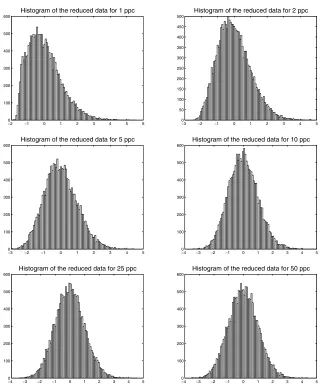
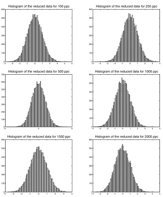
N ). For a normal distribution, we should have on the average: γ₁ = 0 and γ₂ = 0. According to the results recorded in table 2, the extracted noise can be considered as being Gaussian fornppc >50. In spite of the (slight) failure of the Lilliefors test for the 2000 ppc case, we can ascertain the normality hypothesis. Indeed, figure 5 and 6 enable us to visually confirm the Gaussian trend of the distribution. For denoising methods related to non necessarily Gaussian noise, the reader may refer to e.g. to [1] and the bibliography therein.

nppc Lilliesfors’ parameter Skewness coefficient Kurtosis coefficient

1 0.0592 0.8328 0.7759

2 0.0391 0.5292 0.2537

5 0.0265 0.3201 0.0492

10 0.0167 0.2397 0.1008

25 0.0093 0.1398 0.0613

50 0.0074 0.1076 0.0294

100 0.0072 0.0680 0.0027

250 0.0047 0.0240 -0.0061

500 0.0056 0.0322 -0.0329

1000 0.0045 0.0362 -0.0372

1500 0.0046 0.0320 -0.0548

2000 0.0086 0.0363 -0.1165

−2 −1 0 1 2 3 4 5 6 0

100 200 300 400 500 600

Histogram of the reduced data for 1 ppc

−30 −2 −1 0 1 2 3 4 5 50

100 150 200 250 300 350 400 450 500

Histogram of the reduced data for 2 ppc

−3 −2 −1 0 1 2 3 4 5 0

100 200 300 400 500 600

Histogram of the reduced data for 5 ppc

−40 −3 −2 −1 0 1 2 3 4 5 100

200 300 400 500 600

Histogram of the reduced data for 10 ppc

−4 −3 −2 −1 0 1 2 3 4 5 0

100 200 300 400 500 600

Histogram of the reduced data for 25 ppc

−40 −3 −2 −1 0 1 2 3 4 5 100

200 300 400 500 600

Histogram of the reduced data for 50 ppc

Figure 5. Noise distribution for different nppc using histograms with 100 bins. Note that the distributions have been centered and normalized by their variance, i.e. zi= si−_σm

4.

Conclusions and perspectives

−4 −3 −2 −1 0 1 2 3 4 5 0

100 200 300 400 500 600

Histogram of the reduced data for 100 ppc

−50 −4 −3 −2 −1 0 1 2 3 4 100

200 300 400 500 600

Histogram of the reduced data for 250 ppc

−5 0 5

0 100 200 300 400 500 600 700

Histogram of the reduced data for 500 ppc

−40 −3 −2 −1 0 1 2 3 4 5 100

200 300 400 500 600

Histogram of the reduced data for 1000 ppc

−4 −3 −2 −1 0 1 2 3 4 0

100 200 300 400 500 600

Histogram of the reduced data for 1500 ppc

−40 −3 −2 −1 0 1 2 3 4 5 100

200 300 400 500 600

Histogram of the reduced data for 2000 ppc

Figure 6. Noise distribution for different nppc using histograms with 100 bins. Note that the distributions have been centered and normalized by their variance, i.e. zi= si−_σm

respect to the nppc, we observe that it is all the more large, that the nppc is low. As a consequence, we observe strong oscillations in the vicinity of these loci . By incautiously injecting such non physical values in the iterative process, we are led to false solutions. A means to suppress this shortcoming could consist in the use of the so-called translation-invariant wavelets (see [4, 8, 26]). This approach consists in averaging the transform in the vicinity of these regions. After using this method, we observed that the oscillations diminish in amplitude. However, a thorougher study of this stage remains to be achieved both on theoretical and numerical implementation aspects. Last but not least, rigorous comparisons should be made with other types of solvers, in order to validate the quality of such improvements.

Last but not least, since the project was also supported by TU Karlsruhe and ULP Strasbourg, we address our greatest thanks to these institutions.

References

[1] R. Averkamp and Houdr´e,Wavelet thresholding for non (necessarily) Gaussian noise: a preliminary report, CRM Proceedings and lecture notes, vol. 18, Centre de recherches math´ematiques, American mathematical society, 1999, pp. 347–354.

[2] A. Azzalini, M. Farge, and K. Schneider, Nonlinear wavelet thresholding: A recursive method to determine the optimal denoising threshold., Appl. Comput. Harm. Anal.18(2005), no. 2, 177–185.

[3] R. Barthelm´e,Le probl`eme de conservation de la charge dans le couplage des ´equations de Vlasov et de Maxwell, Ph.D. thesis, Universit´e Louis Pasteur, Strasbourg, 2005, (in french).

[4] K. Berkner and R.O. Wells ,Jr.,Smoothness estimates for soft–threshold denoising via translation–invariant wavelet trans-forms, Applied and computational harmonic analysis12(2002), 1–24.

[5] C.K. Birdsall and A.B. Langdon,Plasma physics via computer simulation, Series in plasma physics, Adam Hilger, Bristol, 1991.

[6] J.-P. Chehab, A. Cohen, J. Roche, D. Jennequin, J.J. Nieto, and C. Roland, Solution of Vlasov-Poisson equations using adaptive multiresolution methods, CEMRACS 2003, IRMA Lectures in Mathematics and Theoretical Physics, EMS, pp. 29– 42.

[7] A. Cohen,Numerical analysis of wavelet methods, Elsevier,North–Holland, Amsterdam, 2003.

[8] R.R. Coifman and D. Donoho,Translation–invariant de–noising, Lect. Notes Stat.103(1995), 125–150. [9] I. Daubechies,Ten lectures on wavelets, SIAM, Philadelphia, 1992.

[10] D. Donoho,De–noising by soft–thresholding, IEEE transactions on information theory41(1995), no. 3, 613–627. [11] D. Donoho and I. Johnstone,Ideal spatial adaptation via wavelet shrinkage, Biometrika81(1994), no. 3, 425–455.

[12] D.L. Donoho and I.M. Johnstone,Adapting to unknown smoothness via wavelet shrinkage, Journal of the american statistical association90(1995), no. 432, 1200–1224.

[13] I.M. Dremin, O.V. Ivanov, and V.A. Nechitailo,Wavelets and their use, Physics-Uspekhi44(2001), no. 5, 447–478. [14] M. Farge,Wavelet transforms and their applications to turbulence, Ann. Rev. Fluid Mech.24(1992), 395.

[15] M. Farge, G. Pellegrino, and K. Schneider,Coherent vortex extraction in 3D turbulent flows using orthogonal wavelets, Phys. Rev. Lett.87(2001), no. 5, 45011–45014.

[16] R.J. Goldston and P.H. Rutherford,Introduction to plasma physics, Institute of physics, Bristol, 1995.

[17] Y.N. Grigoryev, V.A. Vshivkov, and M.P. Fedoruk,Numerical “Particle-in-Cell“ Methods, VSP BV, Utrecht,Boston, 2002. [18] J.W. Hockney and J.W. Eastwood,Computer simulations using particles, Institute of physics, Bristol, 1988.

[19] A.J. Jerri,Reducing the Gibbs phenomenon in a Fourier–Bessel series, Hankel and Fourier transform, Contemporary math-ematics190(1995), 179–194.

[20] N.A. Krall and A.W. Trivelpiece,Principles of plasma physics, San Francisco Press, San Francisco, 1986.

[21] H. Krim, D. Tucker, S. Mallat, and D. Donoho,On denoising and best signal representation, IEEE transactions on information theory45(1999), no. 7, 2225–2238.

[22] H.W. Lilliefors,On the Kolmogorov–Smirnov test for normality with mean and variance unknown, J. Am. Stat. Assoc.62 (1967), 399–402.

[23] S. Mallat,A wavelet tour of signal processing, Academic Press, London, 1999.

[24] O. Roussel, K. Schneider, and M. Farge, Coherent vortex extraction in 3D homogeneous turbulence: comparison between orthogonal and biorthogonal wavelet decompositions, J. of Turbulence6(2005), no. 1.

[25] K. Schneider, M. Farge, G. Pellegrino, and M. Rogers, Coherent vortex simulation of 3D turbulent mixing layers using orthogonal wavelets, J. Fluid Mech.534(2005), no. 10, 39–66.

[26] H.-T. Shim,On the Gibbs phenomenon for wavelet expansions, Journal of approximation theory84(1996), 74–95.