Numerical stability of a plasma sheath,,,****

(1)

Laurence CARASSUS, Marion DARBAS, Ghislaine GAYRAUD, Olivier GOUBET, St´ephanie SALMON

NUMERICAL STABILITY OF A PLASMA SHEATH

∗,∗∗,∗∗∗,∗∗∗∗

Mehdi Badsi

1

, Michel Mehrenberger

2

and Laurent Navoret

3

Abstract. We are interested in developing a numerical method for capturing stationary sheaths, that a plasma forms in contact with a metallic wall. This work is based on a bi-species (ion/electron) Vlasov-Amp`ere model proposed in [3]. The main question addressed in this work is to know how accurately classical time-dependent Vlasov-Amp`ere numerical schemes preserve in long time these non-homogeneous stationary solutions with emission/absorption boundary conditions. In the context of high-order semi-Lagrangian methods, due to their large stencil, interpolation near the boundary of the domain requires also a specific treatment.

Résumé. Nous sommes intéressés à développer une méthode numérique pour capturer les gaines stationnaires qu’un plasma forme au contact d’un mur métallique. Ce travail est basé sur un modèle de Vlasov-Ampère proposé dans [3]. La question principale posée dans ce travail est de savoir dans quelle mesure les schémas numériques classiques pour le système Vlasov-Ampère préservent ces solutions stationnaires non-homogènes avec conditions aux bords d’émission/absorption. Dans le contexte de la méthode semi-Lagrangienne d’ordre élevé, à cause du stencil large, l’interpolation près du bord du domaine nécessite aussi un traitement spécifique.

Introduction

When a plasma is in contact with a metallic wall, stationary boundary layers form: they are called plasma sheaths. They are due to both the reflexion/absorption properties of the wall and the charge imbalance coming from the mass difference between electrons and ions: electrons leave the plasma faster than ions. A drop of the self-consistent potential at the wall is indeed built up to accelerate ions and decelerate electrons just as to ensure an equal flux of ions and electrons (a zero current) at the wall. In this work, the starting point is a plasma sheath model proposed in [3]: this is a solution of the stationary Vlasov-Poisson system, whose existence is guaranteed by a so-called kinetic Bohm criterion on the incoming ion distribution. The kinetic distribution in

∗_{This work comes from discussions during the SMAI conference. We thank all the organizers of the conference and also all}

the speakers of the MULTIKIN mini-symposium.

∗∗ _{Thanks to David Coulette, for the discussion and suggestion concerning the boundary conditions.} ∗∗∗_{Thanks to the Selalib team}

http: // selalib. gforge. inria. fr/ and in particular Pierre Navaro

∗∗∗∗ _{This work has been carried out within the framework of the EUROfusion Consortium and has received funding from}

the Euratom Research and Training Programme 2014- 2018 under Grant Agreement No. 633053. Computing facilities were provided by the EUROfusion Marconi supercomputer facility. The views and opinions expressed herein do not necessarily reflect those of the European Commission.

1 _{Institut de Math´}_{ematiques de Toulouse, UMR 5219, Universit´}_{e Toulouse 3, 118 Route de Narbonne, 31400 Toulouse}

2 _{Institut de Recherche Math´}_{ematique Avanc´}_{ee, UMR 7501, Universit´}_{e de Strasbourg et CNRS, 7 rue Ren´}_{e Descartes, 67000} Strasbourg, France, INRIA Nancy-Grand Est, TONUS Project, Strasbourg, France

3 _{Institut de Recherche Math´}_{ematique Avanc´}_{ee, UMR 7501, Universit´}_{e de Strasbourg et CNRS, 7 rue Ren´}_{e Descartes, 67000} Strasbourg, France, INRIA Nancy-Grand Est, TONUS Project, Strasbourg, France

c

EDP Sciences, SMAI 2018

(2)

phase space (position/velocities) for ions and electrons explicitly depends on the potential in the sheath domain, which is solution to a non-linear Poisson equation. The obtained equilibrium is nonhomogeneous in space and involves discontinuities. The stability of its linearized version has been studied in [2].

We here consider the corresponding non-stationary ion/electron Vlasov-Amp`ere model and its numerical implementation through a semi-Lagrangian scheme [7]. Semi-Lagrangian schemes are transport solvers with no stability conditions on the time step: time step is only constrained by the physical dynamics that has to be captured. High-order schemes, using high degree interpolation and time splitting, can be devised and parallel implementation can be considered. We raise here the following questions:

• Question 1: How can we treat boundary conditions with large stencil interpolation ?

• Question 2: How do semi-Lagrangian scheme preserve in time this non-homogeneous equilibrium ? For the first question, fictitious values of the distributions functions will be set at the spatial boundaries, using the so-called butterfly extrapolation method.

For the second question, the discretized stationary solution is not exactly preserved by the time dependent numerical scheme. However, we can expect that the numerical solutions would remain close to the equilibrium. This is actually a numerical stability study. We will see that the equilibrium is numerically stable provided that the incoming current, not exactly zero at the discrete level, is made small. This will be ensured by taking a fine grid in space and velocity and a time step small enough.

Finally, we emphasize that the time step is constrained by the electronic dynamics, that implies stringent restrictions on time and space steps: the preservation of equilibria is all the more difficult to obtain.

1. Sheath model

1.1. Stationary solution

Following [3], we consider a one-dimensional domain [0,1]: particles enter the domain on the left (x= 0) and the metallic wall is located at abscissax= 1. We consider in this work purely absorbing boundary conditions at the wall. The interval [0,1] represents the sheath domain.

Electrons and ions are described by their distribution functions in phase space, denotedfsh

se(x, v) andf sh

si(x, v)

with spatial variable x∈[0,1] and velocity variablev∈R, satisfy the dimensionless stationary Vlasov system:

v ∂xfsshe −

1 µE

sh_∂

vfsshe = 0, (1)

v ∂xfsshi + E sh_∂

vfsshi = 0, (2)

where µ1 is the mass ratio between electrons and ions, andEsh₍_x_{) denotes the stationary electric field. It}

satisfies the Poisson equation:

Esh =−dφ dx sh

, −ε2d 2_φ

dx2 sh

=ρsh, (3)

ρsh(x) =

Z

v∈R

(f_ssh

i(x, v)−f sh

se(x, v))dv, (4)

where φsh(x) is the electric potential,ε1 is the dimensionless Debye length of the plasma andρsh(x) is the charge density.

Boundary conditions. At the entrance of the domain, incoming ions and electrons have distributions:

∀v >0, f_ssh

i(0, v) =f

in

si(v), f sh

se(0, v) =n0 r

2µ π e

−µv 2

(3)

wheren0∈R+is the incoming electron charge density, that will be determined to have a given charge densityρ0

at the entrance of the domain. Thus, electrons have a Maxwellian distribution. At the wall, ions and electrons are supposed here to be totally absorbed :

∀v <0, f_ssh

i(1, v) = 0, f sh

se(1, v) = 0,

The boundary conditions of the potential (3) are defined as follows. The potential values at x= 0 is set to 0 and the potential at the wall, φw =φsh(1), also called floating potential, will be implicitly fixed such that the current vanishes at the wall. Since both electron and ion momentum are constant in space, it amounts to impose that the current vanishes at the entrancex= 0:

Z

v∈R

vf_ssh

i(0, v)dv= Z

v∈R

vf_ssh

e(0, v)dv. (6)

Solutions. Using the characteristic lines of the transport equation and under the hypothesis that the potential is decreasing in the domain, the solution to problem (1)-(2)-(3) is given by:

f_ssh

i(x, v) =1nv>√−2φsh(x)of

in si

q

v2_{+ 2}_φsh₍_x₎_, ₍₇₎

f_ssh

e(x, v) =1nv≥−q2

µ(φsh(x)−φw)

of_sin

e r

v2₋ 2 µφ

sh₍_x₎_, ₍₈₎

where the potential in the sheath domain is the solution to the following non-linear Poisson equation:

−ε2d 2_φ

dx2 sh

(x) =

" Z

R+

fsini(v)v p

v2₋₂_φsh₍_x₎dv #

−√2n0

2π

" √

2π eφsh(x)− Z +∞

√ −2φw

e−v

2 2 v

p

v2_{+ 2}_φsh₍_x₎dv #

, (9)

complemented by the Dirichlet boundary conditions givingφsh(0) andφw=φsh(1):

φsh(0) = 0, (10)

Z

v∈R

vf_sin_i(v)dv=

r

2 πµn0e

φw_, ₍₁₁₎

where the second condition comes from (6) after inserting expressions (8) and (5).

Instead of using the incoming electron densityn0 as a parameter of the problem, we prefer to use the charge

densityρ0=ρsh(0)∈Rat the entrance of the domain, withρsh defined in (4). Using (7)-(8) and (5), we can

expressn0 as a function ofρ0,φwand the incoming ion distribution:

n0= r

π 2

R

v∈R+f in

si(v)dv−ρ0

(√2π−R_√+∞ −2φwe

−v2 2 dv)

, (12)

The problem is then solved in two steps:

(1) when inserting (12) in (11), we obtain the following relation betweenφw andρ0:

1

√ µe

φw Z

v∈R

fsini(v)dv−ρ0

+

Z

v∈R

vfsini(v)dv

Z +∞

√ −2φw

e−v

2 2 _dv

(4)

A negative potential drop at the wallφw≤0 is uniquely defined satisfying (13) provided that the ionic distribution satisfies the relation:

R R+f

in si(v)v dv R

R+f in

si(v)dv−ρ0 ≤

r

2 µπ.

(2) then, once this potential wall exists, the non-linear Poisson equation (9), complemented with the bound-ary conditionsφsh(0) = 0 andφsh(1) =φw, has a unique solution under the kinetic Bohm criterion:

Z

R+

fin si(v)

v2 dv Z

R+

f_sin_i(v)dv <

√

2π+

Z +∞

√ −2φw

e−v2_/₂

v2 dv √

2π− Z +∞

√ −2φw

e−v2/2dv .

Parameters. The equilibria has been computed by the gradient algorithm described in [3] with the following parameters:

• the dimensionless Debye length is set toε= 0.01.

• the charge is zero at the entrance of the domain: ρ0= 0. • the incoming ion distribution is given by

f_sin_i(v) =1{v>0}min(1, v2/η)

1

√

2πσ2e −(v−Z)2

2σ2 , η= 10−1, σ= p

Ti/Te= 0.5, Z = 1.5. (14)

Z is the macroscopic ion velocity when entering the domain.

• the incoming electronic distribution is Maxwellian as given by (5). For the sake of completeness, we recall the expression:

f_sin_e(v) =1{v>0}n0 r

2µ πe

−µv 2

2 , µ= 1/3672. (15)

µis the mass ratio of a deuterium plasma.

Given these parameters, we can compute n0, φw with (13)-(12), and the electric potentialφsh by solving the non-linear Poisson equation (9). In the numerical results, we take :

n0= 0.50191266314760252, φw=−2.7839395640524267.

In practice, for future use in the non-stationary model, we store the nonlinear potentialφsh _{on a uniform grid}

ofN = 2048 cells, that is, at pointsj/N, j= 0, . . . , N.

1.2. Non-stationary model

In the non-stationary setting, electron and ion distribution functions, fse(t, x, v) and fsi(t, x, v), and the

electric field,E(t, x), depend also on timet >0. They satisfy the non-linear Vlasov-Amp`ere system:

∂tfse+v ∂xfse−

1

µE ∂vfse = 0, (16)

∂tfsi+v ∂xfsi+ E ∂vfsi = 0, (17)

(5)

whereJ denotes the current density:

J(t, x) =

Z

v∈R

v(fsi(t, x, v)−fse(t, x, v))dv.

Initial data. The initial data are given by the stationary solution: fse(0, x, v) =f

sh

se(x, v), fsi(0, x, v) =f sh

si(x, v), E(0, x) =E sh₍_x₎_.

We note that the initial electric fieldE(x,0) satisfies the following Poisson equation:

ε2∂xE(0, x) =nsi(0, x)−nse(0, x), (19)

Z 1

0

E(t, x)dx=−φw, (20)

where the densitiesnsi andnse are given by:

nse(t, x) = Z

v∈R

fse(t, x, v)dv, nsi(t, x) = Z

v∈R

fsi(x, v)dv,

andφw is the floating potential atx= 1.

2. Numerical scheme

We solve system (16)-(17)-(18) using a semi-Lagrangian scheme. Due to the large mass ratio between electrons and ions, the computational domain of electrons will be larger than the ion one and thus velocity meshes have to be different for the two kinds of particles.

Mesh notations. We consider uniform cartesian meshes for both spatial domain [0,1] and velocity domain [vmin, vmax]. Considering Nx+ 1 points in the spatial direction and Nv+ 1 points in the velocity one, mesh points are denoted (xi, vj) = (i∆x, vmin +j∆v) for all 0 ≤ i ≤ Nx and 0 ≤ j ≤ Nv with ∆x = 1/Nx and ∆v = (vmax−vmin)/Nv. Note that the definitions relative to the velocity domain implicitly depend on the particle s∈ {se, si} under consideration. We denote by fs,n(i,j) the approximate value of the distribution

functionfs at point (xi, vj) at time tn =n∆t, with ∆t >0 andn∈N, andEin the approximate value of the electric field at pointxi.

2.1. Initialization of the electric field

The solution to system (19)-(20) is given by:

E(x) =

Z x

0

nsi(y)−nse(y)

ε2 dy−φw− Z 1

0 Z x

0

nsi(y)−nse(y)

ε2 dydx. (21)

The charge densitiesns, s∈ {se, si}are computed at grid pointsxiusing the trapezoidal formula in the velocity direction from the distributions functions1. We then consider a reconstruction at any pointx=xi+α∆x∈[0,1], withα∈[0,1], by local centered Lagrange interpolation of degree 2d+ 1 withd∈N:

ns,h(x) = d+1 X

k=−d

ns,i+kLk(α),

1_{The trapezoidal formula is spectrally accurate for smooth periodic data and remains accurate when the velocity domain is large}

(6)

whereLk are the elementary Lagrange polynomials:

Lk(α) = d+1

Y

i=−d i6=k

(α−i)/(k−i). (22)

Note that the densities have to be defined at points outside of the domain whend > 0. This will be done by expanding the definition of the distribution functions. This point will be detailed in Section 2.3. The discrete electric field at grid pointsxi is then obtained from (21) in whichnsare replaced by their discrete counterparts ns,h. The involved integrals are computed exactly and the overall scheme hasO(∆x2d+2) accuracy.

2.2. Splitting

To solve the Vlasov-Amp`ere system, we use a splitting between space and velocity dynamics and write it as a succession of one-dimensional advections. More precisely, we consider the following dynamics: the kinetic transport system given by:

(T) ∂tfse+v ∂xfse = 0, (23)

∂tfsi+v ∂xfsi = 0, (24)

ε2∂tE=−J, (25)

and the electric transport system, given by:

(U) ∂tfse−

1

µE ∂vfse= 0, (26)

∂tfsi+E ∂vfsi = 0, (27)

ε2∂tE= 0. (28)

Since the electric field is constant in time in this second step, both dynamicsT andU are advections at constant velocities. In practice, to obtain second order accuracy in time, we consider the Strang splitting which consists in computing fors∈ {se, si}

f_s,n+1₍_i,j₎ i,j

,(E_in+1)i

=hUh,∆t/2◦ Th,∆t◦ Uh,∆t/2 i n

(f_s,n₍_i,j₎)i,j,(E_in)io

whereTh,τ andUh,τ are discrete approximations ofT andU over a time intervalτ (withτ= ∆torτ= ∆t/2). Each transport equation is solved using a semi-Lagrangian scheme with centered Lagrange interpolation of degree 2d+ 1. We thus consider the discretized version of the kinetic and electric transport dynamics. Operator

Th,τ : ((fs,(i,j)),(Ei)i)→((fs,∗(i,j)),(Ei∗)i) consists in the following: for any grid points (xi, vj), we define the shifted indexi∗ andα∈[0,1] such thatxi−vjτ =xi∗+α∆xand then the distribution function is given by:

f_s,∗₍_i,j₎= d+1 X

k=−d

fs,(i∗₊_k,j₎L_k(α),

where the (Lk) are defined in (22), and the electric field at point xi is given by:

E_i∗=Ei− τ ε2

Ji+Ji∗ 2 ,

(7)

the grid points, starting from the interpolated distribution function in the spatial direction, while the Amp`ere equation (25) is computed using a second order Crank-Nicolson scheme. The interpolation requires values of the distribution function outside the domain: we explain in the next section how to extrapolate it.

OperatorUh,τ : ((fs,(i,j)),(Ei)i)→((fs,∗(i,j)),(E ∗

i)i) consists in the following: for any grid points (xi, vj), we define the shifted indexes js∗i, j

∗

se and αsi, αse ∈[0,1] such that vj−Eiτ =vj_si∗ +αsi∆vsi and vj+ 1

µEiτ = vj∗

se +αse∆vse and then

f_s,∗₍_i,j₎= d+1 X

k=−d fs,(i,j∗

s+k)Lk(αs),

E_i∗=Ei.

For this advection in velocityUh,τ, periodic boundary conditions are used; we have here made the presentation for Lagrange interpolation, as it is used for advection in space, but other advection scheme can be used; in particular, in the numerical results, we will use cubic splines.

2.3. Boundary conditions

In both the initial computation of the electric field and the advection in spaceTh,τ, the proposed numerical scheme requires to take values of the distribution function outside the physical domain.

For anyxi=i∆x <0 andvj, we consider the following extrapolation at the entryx= 0:

fs,(i,j)= (

fs(0,0, vj), ifvj≥0,

2fs,(0,j)−fs,(−i,j), ifvj<0.

For anyxi+Nx= (i+Nx)∆x >1 andvj, we consider the following extrapolation at the wallx= 1:

fs,(i+Nx,j)= (

2fs,(Nx,j)−fs,(Nx−i,j) ifvj ≥0,

0 ifvj <0 .

This corresponds to a purely Dirichlet condition for incoming velocities and an extension by imparity for leaving velocities (also calledbutterfly procedure).

3. Numerical results

3.1. Sheath test-case

We here used the following set of parameters:

d= 8, Nx= 2048, Nv= 4096,

velocity domain [−200,500] for electrons and [−5,5] for ions, (29)

∆t= 10−5.

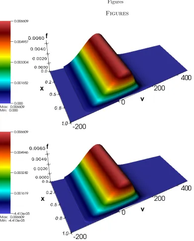
The simulation has run on 256 processors during 24 hours, with final time t = 8.03478, on the Marconi supercomputer; the distribution function is stored every multiple of 0.01, and the time diagnostics every time step.

(8)

to be not crucial here, as it is not far from being preserved and it can be used as a measure of accuracy of the simulation as other theoretically preserved quantities. We see that the distribution function of electrons presents a discontinuity; this has the effect that the quadrature in velocity for computing the current converges slowly, and thus a high number of points in velocity is needed.

For ions, we see that the distribution is not constant in space near the wall (x= 1) for a given velocity. At this boundary, the butterfly procedure does not destroy theC1 _{property of the distribution function and seems}

to be more adapted than the prolongation by a constant value, which is used for incoming velocities. Note also that the fictitious boundary values are only used to interpolate inside the domain, as the sub time stepτis here always positive (negative time steps, could be however considered when going to higher order splitting schemes in time, but are not studied in this work).

The space discretization is rather fine; this is needed for the sharp gradient near the wall. Non-uniform grids could be useful here to save memory and computations [5], but are not tackled here for simplicity. We mention also that high order interpolation is used, which permits not to have to refine too much. High order schemes in a non uniform setting could be considered with a Semi-Lagrangian Discontinuous Galerkin method (SLDG) (see [6], for example), or with non uniform cubic splines (see for example [1]).

Finally, we note that the time step is chosen very small. The time-scale of the electron oscillations are characterized by the so-called plasma frequency ωp = 1/(ε

√

µ) (where ε is the Debye length and µ the mass ratio). In order to capture these oscillations, the time step should be indeed smaller than 1/ωp '1.6·10−4. However, as we are interested in studying the stability of the equilibrium for long times (at least long with respect to the electron dynamics), we have to reduce the time step to one order of magnitude in order to reduce the time error (due to the Strang splitting and the Crank-Nicolson scheme for the Amp`ere equation). Here again, higher order schemes in time might be useful, in order to use larger time steps (see for example [1]).

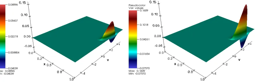
On Figure ?? (resp. ??), we represent the difference between the distribution function of electrons (resp. ions) at time 0 and at time t= 4 and t = 8. We see that the error for the electrons is mainly localized near the wall and at the discontinuity of the distribution. As regards ions, the error is localized near the wall. We see that the error near the wall increases in time, especially for the ions. We remark also an exceptional value for the electrons, that seems to be located at v = 0 and x= 1: this might be explained by the fact that the function is not modified by the space advection (atv= 0), and is thus not diffused.

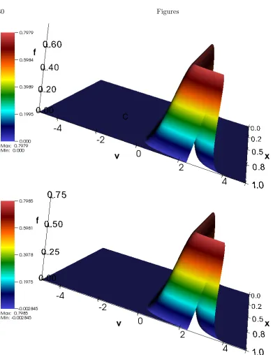
On Figure ??, we represent 2d views of the distribution function of electrons and ions at time t = 8. We recognize here the pictures of [3].

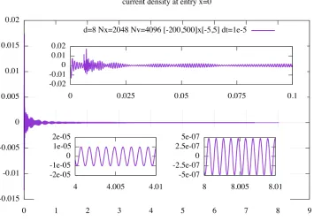
Current density at the entry. On Figure??, we represent the current density at the entry x= 0 (which is zero at the continuous level). We expect a better behavior on the this boundary than at the wall, where the convergence is more delicate. We remark an oscillatory behavior due to the electron dynamics. After aviolent behavior at time around 0.01, where the value can have a peak around 0.02 (that value is guessed to be linked to the space discretization), it tends to decrease and stabilize, while still oscillating around 0, with the same frequency.

Other diagnostics. On Figure?? (left), we represent the total energy, whose continuous expression is

E(t) =µ 2

Z

v∈R Z 1

0

v2fse(t, x, v)dxdv+

1 2

Z

v∈R Z 1

0

v2fsi(t, x, v)dxdv+

ε2

2

Z 1

0

E2(t, x)dx.

The time evolution of this quantity a priori depends on the boundary terms. However, for the test-case under consideration, this quantity should be conserved since we would like to capture a stationary solution. Except at the very beginning, it is decreasing and reaches a relative error of about 0.02% at final time. Similarly, the total charge:

ρtot(t) = Z 1

0

(ni(x, t)−ne(x, t))dx,

(9)

We then represent the time evolution of total density and L1 _{norm of the distribution function}2 _{for ions}

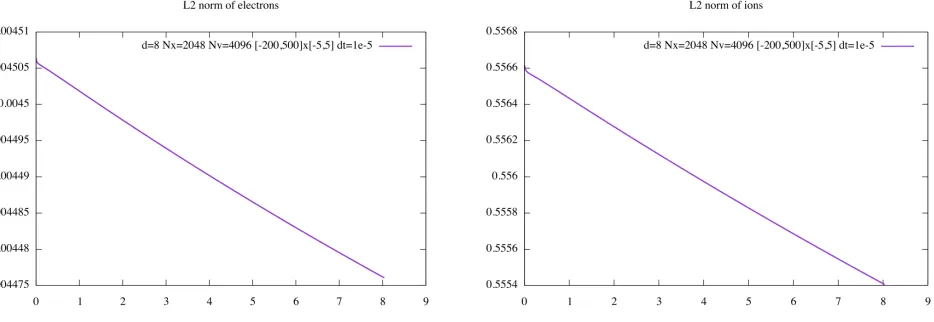
and electrons on Figure??and theL2 _{norm of the distribution function on Figure}_??_{. We see that their time}

behavior is similar to the total energy one. Note that the L1 _{norm and total density are indistinguishable (for}

both ions and electrons), which shows that the positivity of the distribution functions is rather well preserved.

3.2. Comparison with other numerical boundary conditions

The butterfly procedure has been introduced to extrapolate the values of the distribution function and then keep the centered interpolation even when the interpolation stencil involves points outside the computational domain. Instead, we could have considered to always use grid points and thus consider non-centered interpolation at the boundaries (with the 2d+ 1 nearest points to the boundary). This would have the advantage to keep the same order of spatial approximation at the boundaries. However, we see on Figure ??(left) that this method leads to unstable results: the total energy blows up ford= 4 andd= 5 and the blow-up happens sooner when the degree is large. For d = 1, which corresponds to interpolation degree equal to 3 and requires only one extrapolation point, the solution remains stable on the time interval under consideration but may give rise to instabilities in large time. On Figure??(right), we compare two implementations of the unstable method: the times of blow-up are the same and this guarantees that the unstable method is correctly implemented. Finally, we mention that semi-Lagrangian schemes with Lagrange interpolation has been proved stable and convergent only with centered interpolation [4].

3.3. Comparison with other parameters

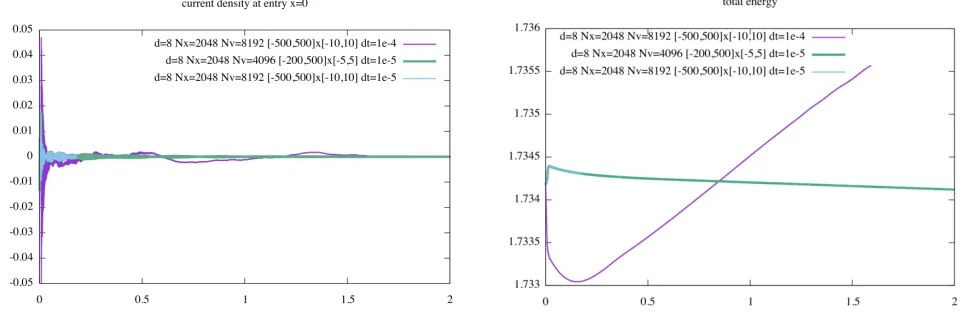
On Figure??, we show how the numerical results change when enlarging the computational domain in velocity (taking velocity domain [−500,500] for electrons and [−10,10] for ions andNv = 8192), and then increasing the time step (∆t= 10−4 _{instead of ∆}_t_{= 10}−5_{). We compare the current density at the entry}_x_{= 0 and the}

total energy. We observe that the change in velocity domain has no influence, while the change in time step ∆t leads to less accurate results.

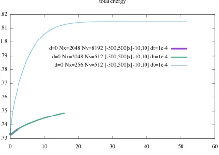
On Figure??, we present the results when taking less discretization pointsNx= 256,Nv= 512 and velocity domain [−500,500] for electrons and [−10,10] for ions and ∆t = 10−4. This enables to consider longer time simulation, but we see that the results are degraded especially in large time.

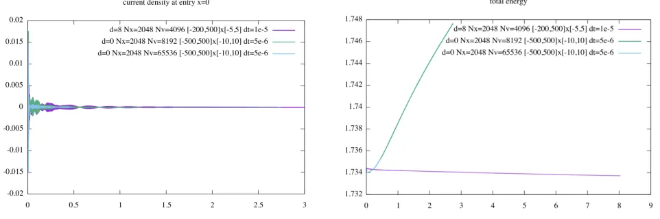
On Figure ??, we consider low order interpolation d = 0. Note that in this case, there is no need of extrapolated values and the butterfly procedure is not active. We consider ∆t = 5·10−6 and Nv = 8192 or Nv = 65536. The velocity domain are [−500,500] for electrons and [−10,10] for ions. We see that the current density at the entry x= 0 is improved when using more points in velocity. This is however not true as regards the other diagnostics: the case d= 0 leads to an increase of the total energy of about 0.8% at timet= 3 and can not compete with the high order scheme, which require butterfly extrapolation procedure.

On Figures ?? and ??, we consider the case d = 0, with ∆t = 10−4 _and _N

x = 256 or Nx = 2048 and Nv= 8192 orNv = 512. Comparing with the previous case withd= 8 (Figure??), we see that there is no such oscillatory behavior in large time. However, forNx= 256 and Nv= 512, we see that the increase of the total energy is about 4.5% and it leads to different behaviors: the current density at entry tends to a value around 0.1 instead of 0.

4. Conclusion

We have studied the behavior of the numerical solution of the Vlasov equation, initialized with a sheath equilibrium [3]. The numerical results show that the difference between the numerical electronic distribution and the initial condition remains bounded in time. This is in agreement with the linear stability result obtained in [2], which states that, in the absence of perturbation on the ionic distribution and in the linear regime, the perturbation on the electronic distribution remains bounded over time. As pointed in section 3.2, the

2_{Total density is given by:} R v∈R

R1

0 fs(t, x, v)dxdv =

R1

0 ns(t, x)dx. L1 norm of the distribution function is given by:

R v∈R

R1

(10)

discretization of the boundary condition is crucial as using non centered Lagrange interpolation could lead to instabilities. Thanks to high resolution in velocity, high order interpolation and very small time steps, we are able to recover the equilibrium accurately for relatively long time compared to the electronic time scale. This work is a first step as regards the numerical method. We mention here several directions of research:

• to reduce the constraint on the time step, asymptotic preserving schemes could be designed, the fictitious boundary values may be improved and we could consider unsplit time integration,

• to reduce the constraint on space/velocity grid, adaptive/Discontinuous-Galerkin method or delta-f method could be considered,

• scheme ensuring a discrete Gauss law could be develop and its impact on the numerical results could be analyzed,

• we could enhance mixed openmp/mpi parallelization to get full performance on current and future architectures.

References

[1] B. Afeyan, F. Casas, N. Crouseilles, A. Dodhy, E. Faou, M. Mehrenberger, and E. Sonnendr¨ucker,Simulations of kinetic electrostatic electron nonlinear (keen) waves with variable velocity resolution grids and high-order time-splitting, The European Physical Journal D, 68 (2014), p. 295.

[2] M. Badsi,Linear electron stability for a bi-kinetic sheath model, Journal of Mathematical Analysis and Applications, 453 (2017), pp. 954 – 972.

[3] M. Badsi, M. Campos Pinto, and B. Despr´es,A minimization formulation of a bi-kinetic sheath, Kinet. Relat. Models, 9 (2016).

[4] N. Besse and M. Mehrenberger,Convergence of classes of high-order semi-lagrangian schemes for the vlasov–poisson system, Mathematics of computation, 77 (2008), pp. 93–123.

[5] D. Coulette and G. Manfredi,An Eulerian Vlasov code for plasma-wall interactions, Journal of Physics: Conference Series, 561 (2014).

[6] N. Crouseilles, M. Mehrenberger, and F. Vecil, Discontinuous Galerkin semi-Lagrangian method for Vlasov-Poisson, ESAIM: Proc., 32 (2011), pp. 211–230.

(11)

Figure Captions

Figure 1. Distribution function of electrons at timet= 0 (top) andt= 4 (bottom). Parameters given in (29).

Figure 2. Distribution function of ions at timet= 0 (top) and t= 4 (bottom). Parameters given in (29).

Figure 3. Error on the electron distribution function, fse(0, x, v)−fse(t, x, v), at timet = 4 (left) and t= 8

(right). Parameters given in (29).

Figure 4. Error on the ion distribution function, fsi(0, x, v)−fsi(t, x, v), at timet= 4 (left) andt= 8 (right).

Parameters given in (29).

Figure 5. Distribution function of electrons (left) and ions (right) at timet= 8. Parameters given in (29).

Figure 6. Time evolution of current densityJ(t, x= 0) at the entryx= 0 and zoom on time intervals [0,0.1], [4,4.01] and [8,8.01]. Parameters given in (29).

Figure 7. Time evolution of total energyE(t) (left) and total charge ρtot(t) (right). Parameters given in (29).

Figure 8. Time evolution of total density andL1 _{norm of the distribution function for electrons (left) and ions}

(right). Parameters given in (29).

Figure 9. Time evolution ofL2_{norm of the distribution function for electrons (left) and ions (right). Parameters}

given in (29).

Figure 10. Time evolution of total energyE(t). Left: Comparison of the butterfly procedure and the uncentered interpolation at the boundary for d= 1,d= 4 andd= 5. Right: Comparison of two implementations of the uncentered interpolation (uncentered: compute extrapolate values using on the interpolating polynomial on the 2d+ 1 nearest points of the boundary and then use the same algorithm as the butterfly procedure, uncentered implem2: direct implementation of the interpolation).

Figure 11. Comparison of the current density at the entry x = 0 (left) and total energy (right) changing ∆t= 10−5 to ∆t= 10−4.

Figure 12. Comparison of the current density at the entry x = 0 (left) and total energy (right) changing ∆t= 10−5 _{to ∆}_t_{= 10}−4 _and_N

xto 256 andNv to 512.

(12)

Figure 14. Current density at the entryx= 0 for d= 0, ∆t = 10−4 _{and different space/velocity parameters}

(left: on short time; right: on long time)

(13)

Figures

Figure 1. Distribution function of electrons at time t= 0 (top) andt= 4 (bottom).

(14)

Figure 2. Distribution function of ions at timet= 0 (top) and t= 4 (bottom). Parameters

(15)

Figure 3. Error on the electron distribution function,fse(0, x, v)−fse(t, x, v), at timet= 4

(left) andt= 8 (right). Parameters given in (29).

Figure 4. Error on the ion distribution function,fsi(0, x, v)−fsi(t, x, v), at time t= 4 (left)

andt= 8 (right). Parameters given in (29).

Figure 5. Distribution function of electrons (left) and ions (right) at time t= 8. Parameters

(16)

Figure 6. Time evolution of current densityJ(t, x= 0) at the entryx= 0 and zoom on time

intervals [0,0.1], [4,4.01] and [8,8.01]. Parameters given in (29).

Figure 7. Time evolution of total energyE(t) (left) and total chargeρtot(t) (right). Parameters

(17)

Figure 8. Time evolution of total density andL1norm of the distribution function for electrons

(left) and ions (right). Parameters given in (29).

(18)

Figure 10. Time evolution of total energy E(t). Left: Comparison of the butterfly

proce-dure and the uncentered interpolation at the boundary for d= 1, d = 4 and d = 5. Right: Comparison of two implementations of the uncentered interpolation (uncentered: compute ex-trapolate values using on the interpolating polynomial on the 2d+ 1 nearest points of the boundary and then use the same algorithm as the butterfly procedure, uncentered implem2: direct implementation of the interpolation).

Figure 11. Comparison of the current density at the entryx= 0 (left) and total energy (right)

(19)

Figure 12. Comparison of the current density at the entryx= 0 (left) and total energy (right) changing ∆t= 10−5to ∆t= 10−4andNx to 256 andNv to 512.

Figure 13. Comparison of the current density at the entryx= 0 (left) and the total energy

(20)

Figure 14. Current density at the entry x = 0 for d = 0, ∆t = 10−4 and different

space/velocity parameters (left: on short time; right: on long time)

Numerical stability of a plasma sheath*,**,***,****