IJST, Transactions of Electrical Engineering, Vol. 37, No. E1, pp 17-33 Printed in The Islamic Republic of Iran, 2013
© Shiraz University
A NOVEL APPROACH TO MEASURING NODE AND ENERGY UNIFORMITY
FOR THE OPTIMAL ASSIGNMENT OF DIRECTIONAL SENSORS
*M. HOSEINI,
**M. DEHGHAN AND H. PEDRAM
Dept. of Computer Engineerin, Amirkabir University Tehran, I. R. of IranEmail: [email protected]
Abstract– One of the prevalent methods to increase the network lifetime is to develop the uniformity in the sensor node distribution and load balancing. The existing criteria to calculate the uniformity are only able to locally or globally measure the uniformity of sensor distribution in the network. In this paper, a new criterion is proposed for the uniformity measurement of sensor distribution. The criterion can calculate the both global and local uniformity in various levels of node distribution. In addition, using the model of sensing area of each sensor, this criterion has been generalized for the uniformity of sensors energy distribution in the network via calculating the uniformity of sensor node distribution. In order to assess the performance of the proposed criterion, a set of sensor distribution patterns has been utilized; also, the uniformity calculation results of these patterns have been studied. Then, a method for the sensor assignment has been proposed in a network, in which sensor nodes have the possibility of rotation and a coverage area is selected. This method enhances the energy distribution uniformity in the network. The comparison is finally provided among the perceived results to show an acceptable performance of the proposed method.
Keywords– Uniformity measurement, global uniformity, local uniformity, directional sensor networks, uniformity maximization
1. INTRODUCTION
Directional Sensor Networks (DSNs) typically consist of numerous nodes. Each node is equipped with directional sensors such as video cameras, processing ability, wireless communication, and relatively limited energy resources, which are distributed in the network area [1]. Deterministic distribution and regular deployment of sensors in the network is often neither feasible nor practical [2]. Generally, sensors are distributed in the sensor network randomly. According to their applications and applied methods, the distribution of sensors can be uniform as Gaussian, Poisson, and so on. In the directional sensor networks, sensors have a limited field of view [3] and their angle can normally modify horizontally [4, 5]. Thus, they could select their coverage area in such a way that energy is distributed uniformly in the entire network region. A uniform sensor node distribution in the wireless sensor network would lead to better and more equitable expenditure of energy in nodes. Consequently, an appropriate criterion to estimate the useful lifetime of the network is uniformity in the network topology. Moreover, it is more likely to cover a desirable area with fewer nodes in a network with the uniform sensor distribution [6]. Uniformity has been defined in some works as the average local standard deviation of the distances between neighbor nodes. Also, it should be noted, this criterion produces some unacceptable results in the measurement of global uniformity.
In this paper, first, a new criterion is introduced for evaluating the distribution uniformity of nodes throughout the network either locally or globally. Instead of the global uniformity that is computed from information of the local uniformity, the Local uniformity is measured by a distributed and an efficient algorithm with minimum communication between neighbor sensor nodes. This is an important reason for computing the local uniformity. Furthermore, the calculation criterion of the uniformity of the node distribution in the network is generalized to calculate the uniformity of the node energy distribution. For this aim, the sensing area model for every single sensor has to be considered as well. In order to evaluate the performance of this criterion, a set of sensor distribution patterns has been proposed. Each pattern is significantly different from others in terms of local and global. Additionally, the uniformity and intuitively of this pattern will be shown to prove the uniformity can be evaluated accurately by using this criterion. It is important to note that in the case of equal energy of the sensor nodes and uniform distribution of nodes, the energy distribution has no uniform distribution in the network area. Also, regions in the center area usually have more energy than regions in the boundaries of the network. An algorithm has been presented to calculate the uniformity of the node distribution in the network in a variety of levels (including global and local) with different scales of regions. This algorithm can measure the local uniformity as distributed and scalable. Based on the information of local uniformity, the algorithm hierarchically calculates the middle uniformity and general uniformity as well. In the following, these sensor nodes have been distributed in a network randomly so they have a specific fixed position, also, they can rotate and alter their sensing coverage angle. Here a method has been proposed to increase this uniformity of energy distribution. Furthermore, this algorithm can do the sensor assignment by different levels of uniformity.
Our contributions in this paper are to meet the goal of prolonging network lifetime, which can be summarized as: 1- Uniformity measurement of the geographical distribution of nodes in multi granularity levels from the local uniformity to the global uniformity instead of the other works in this context which usually concentrate on only one level. 2- Uniformity of energy distribution in regions of the network area is measured again in the multi granularity level. Meanwhile, the assignment of sensors energy to energy of the network regions has been little studied in the other researches. 3- Introducing a distributed and hierarchical algorithm for computing uniformity. 4- Introducing a distributed and hierarchical sensor assignment algorithm for the uniformity maximization.
The organization of this paper is as follows:
In the next section, the accomplished researches in this field are reviewed. A criterion is proposed to measure the uniformity of the node distribution in section 3. It is utilized to present an algorithm for the calculation of uniformity in various levels from the local to global uniformity. In the fourth section, the criterion of uniformity measurement is generalized in order to measure the uniformity of energy distribution instead of the node distribution. In section 5, a sensor assignment algorithm is proposed using the uniformity criterion of energy distribution. In the first step, two models of omni-directional and directional sensor coverage are attended. In addition, the sensors rotational ability is considered. Also, a new method is proposed to enhance the uniformity of energy distribution in the network by consideration of the outcome results of the mentioned issues. This method is able to assign sensors to the network regions in such a way that the energy of the network regions is uniformly distributed. The simulation and performance evaluation of the proposed algorithms are described in section 6. Finally, Section 7 is dedicated to the conclusion and suggestions for future researches.
2. RELATED WORKS
A novel approach to measuring node and…
June 2013 IJST, Transactions of Electrical Engineering, Volume 37, Number E1
19
wireless sensor networks, such as time scheduling, selection of active sensors [7], traffic control, and routing [8]. Based on [9], several methods have been studied for k-coverage boundary problem. Therefore, the application of uniform energy consumption criterion has ended in the best response and it has increased the network lifetime.
In addition, a transmission distance is applied to adjust transmitter energy in wireless sensor networks [10]. To balance the energy consumption, low and high energy sensors are used for communication between near and far distances, respectively.
Furthermore, the existing nodes in the network are divided into several independent sets in such a way that each set could cover the whole network area [7]. A weighted coefficient is attributed to these sets in accordance with the available energy in the set. In order to deal with the coverage issue in each stage, a sensor set is utilized that has a higher amount of energy. Therefore, the constant energy consumption will help to increase the network lifetime.
According to the opinion of Lee et al [11], to balance energy consumption, a set of generated topologies should be used instead of a single given topology for the network during communication between sensor nodes. Each topology is applied on data collection cycles. Therefore, the energy consumption is balanced in the time domain to induce feasibility for the load distribution through various routes (spatial load balancing) as well (temporal load balancing).
All the sensors are able to move in a network for the uniform distribution, so the idea of moving nodes from the regions with the high-density node distribution to the low-density ones can be used. There is a method for inventing sensors deployment in an idea of spreading molecules in physics as well [12]. For this purpose, assuming that there is no global information from the network, an algorithm, called Self-Deployment by Density Control (SDDC), is presented to create a balance between sensors density. Some specifications of this algorithm are provided: simultaneous movement of several sensors, distributed performances, local calculation, and self-deployment. A distributed algorithm has been proposed in [6] for self-deployment of the moving sensors for applying the idea of the repulsion force between charged atoms. The efficiency criteria of this algorithm are as follows: coverage, uniformity, time, the passed distance by nodes and the time of algorithm convergence. Furthermore, the presented algorithm has been compared with an algorithm that includes a node deployment based on the simulated annealing. The uniformity criterion has been defined as the uniform deployment of node positions in the network. According to the sensors coverage area with the aim of k-coverage of targets, the number of sensors that could cover that area is calculated based on each part of the coverage area. The purpose of studying this issue is to realize whether or not it would be possible to cover all the given points with at least k sensors [13].
In the directional sensor networks, added to all the above-mentioned methods, the uniform energy consumption could be controlled in the network for using the sensors rotational capability for sensing the area selection. Moreover, in video sensor networks the energy consumption of sensing is independent to the distance and the presence or absence of targets, also the distance of targets does not have any effect on the energy consumption. In a video sensor, maximum distance of sensing is limited by which targets can be observed with minimum resolution. By aid of these capabilities, high-energy sensors can be applied on coverage of several near and far areas. Use of this capability is one of the innovative issues in this article.
area has been partitioned into a set of small equal-sized parts. In each part, number of available sensors is counted and saved in the weighed grid matrix (WGM). The value of WGM for each region is applied as the sensor selection criterion in such a way that sensor distribution would end in more uniformity. The size of these parts is very small as the sensor located in each part can cover that area.
In [18], a very simple model has been applied to measure the global uniformity of sensor distribution in the network. The network area has been split into four equal regions and the uniformity is explained in terms of number of sensors in each region based on the quality of uniformity in three levels of good, intermediate, and weak.
- Good distribution: There are four states: a) At least two sensors are positioned in each region. b)
Size of the largest area with no sensor is (maximum) ¾ of the whole area. c) Sensors are not centralized in the center or edges. d) The length to width of low-density areas is not larger than 2 to 1.
- Intermediate distribution: There are three states: a) At least one sensor is positioned in each
region. b) Size of the largest area with no sensor is (maximum) equal to the whole area. c) The length to width of low-density areas is not larger than 3 to 1.
- Weak distribution: The remained states are categorized in this segment.
In [15], several criteria are shown for the uniformity measurement of sensor distribution in the network region (such as distance-measure index, area-ration index, clustering index, and U-measure index). Each of them is able to describe the uniformity of sensor distribution in the network. However, each may encounter difficulties in some special conditions. For instance, the U-measure criterion is determined with the following equations.
(1)
N i
i
U N U
1
1
where:
(2)
2 12 1,
1
i
K
j
i j i i
i D M
K U
The variables in these equations are as follows:
N: Total number of nodes
Ki: Number of neighbors of the ith node
Di,j: the distance between the ith and jth node
Mi: the average distance between the ith node and its neighbors
Ui: local uniformity, it is calculated in each sensor for its neighbors U: Total uniformity that is centrally calculated based on local uniformities
Only neighbor nodes in the communication radius are used to calculate local uniformity. It is presumed that communication radius is twice the sensing radius. Therefore, the uniformity criterion is a
local criterion and every node is only able to access the local information. The low value of Ui s and U
would reflect the uniform distribution in the network. The major problem of this criterion refers to the fact
that if all neighbor nodes are in the same distance from the node, U will be zero and the highest amount
uniformity is achieved, i.e, in the mentioned equations, the average distance value does not affect uniformity. For example, in case all of the nodes are located on each other with zero distance, it is still mistakenly interpreted as the maximum uniformity. It should be added that although this criterion is suitable for small-sized areas, it does not perform properly in the entire network area [15].
Vazquez-A novel approach to measuring node and…
June 2013 IJST, Transactions of Electrical Engineering, Volume 37, Number E1
21
Grande (2006), and Justel, Pena and Zamar (1997). In the following a criteria is introduced that can measure the uniformity of distribution of a random multivariate variable. The criterion is as shown bellow:
(3)
, ,…, , ∑ ∑ … ∑ ∏
where
⋮ is a random sample from a k-dimensional population distribution.
The range of Eq. (3) is in [0-1]. It is equal to zero for the total uniform distribution and to one for the total non-uniform distribution.
3. THE CRITERION FOR MEASUREMENT OF THE UNIFORMITY OF NODE DISTRIBUTION
In this section, a criterion is shown for measurement of the uniformity of the node distribution in the network. It is able to calculate the uniformity in different levels. These levels could measure the local uniformity of very small-sized areas as well as the global uniformity of the whole network.
According to the following equation, assume that the network area has been divided into N
equal-sized regions. Total number of nodes in the network is Ns. Nsi, (1≤i≤N) is number of available nodes in each region. The uniformity criterion is obtained from unbiased variance (var(Nsi)).
(4)
% 100 1 1 1 ) var( 1
1 )
,
( 2
N N N Ns N
N N N U
i s
s
In the appendix 1, the selection reasoning and calculation method of this equation are expanded. In this equation, the minimum uniformity value is equal to zero for entirely non-uniform distribution and its maximum value is 100% for completely uniform distribution.
a) The definition of local and global uniformity
Local uniformity: in order to maintain local uniformity, node distribution in small regions of the network
has to be uniform. The most appropriate small region can be regarded in the area under the node communication coverage.
Global uniformity: node distribution should be uniformed in large regions of the network. A region
whose area is a quarter of the whole network can be considered as the large region.
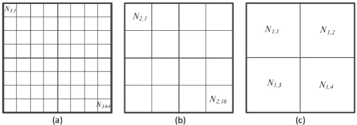
In Fig. 1, the network regions divisions can be seen in three levels. In Fig. 1a small regions are suitable for local uniformity measurement. Figure 1c is appropriate for the global uniformity measurement of large regions. Fig. 1b is good for regions with a size in between.
The algorithm of the uniformity measurement:
In this section, an algorithm is proposed to calculate the uniformity in different levels. Its parameters and notations are described in detail as follow:
l, 1≤l≤L is the area of uniformity calculation. l=1 refers to the largest region and l=L relates to the smallest one. L is the maximum number of levels for uniformity calculation.
Nl,j: Number of sensors in the lth uniformity level and jth region area, where 1≤l ≤L , 1≤j ≤22l. Note
that number of regions in the lth uniformity level is equal to 22l. For example, in the largest
The proposed algorithm stages are provided below.
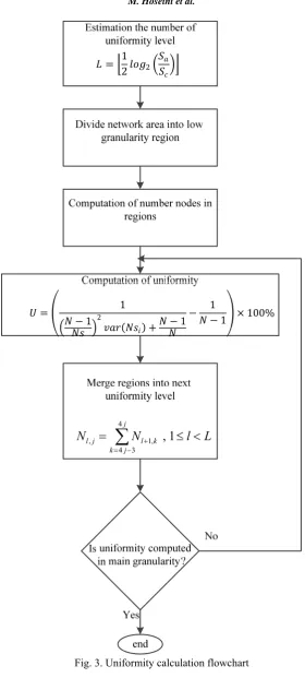
1. Estimation of number of levels for L uniformity calculation: If the area of the smallest and largest
regions are considered equal to communication radius of nodes and a quarter of the entire network area, respectively, for number of uniformity calculation levels, the equation below can be regarded:
(5)
c a
s s L 2log2
1
In this equation, Sa is the network area and Sc is the coverable area for each sensor.
2. Division of the network into small regions with low granularity
3. Count number of nodes in every region for l=L
4. Uniformity calculation of node distribution obtained from Eq. (4)
5. Merger of the network regions: creating areas with the higher granularity and calculating number of
nodes in each region based on the number of included nodes.
(6)
L l N
N j
j k l k j
l
1 , 4
3 4 1, ,
6. Repetition of stages 4, 5, and 6 in order to reach the highest granularity in the network
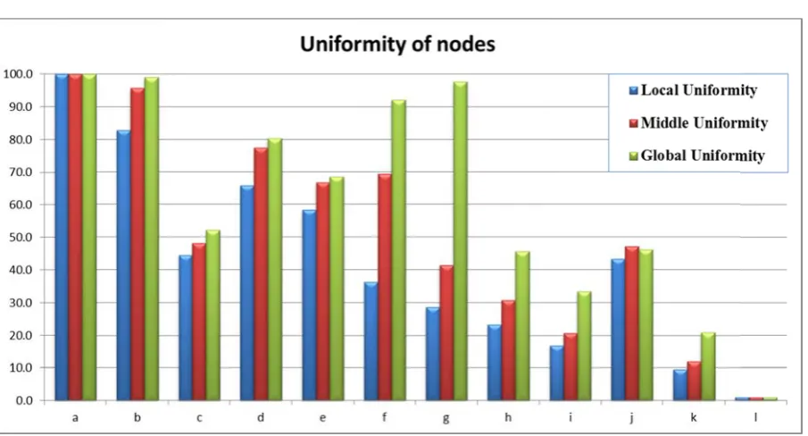
In Fig. 3, the flowchart of the algorithm is shown. Based on the Table 1 and Fig. 2, the results of uniformity measurement are represented using Eq. (4) on several samples of the node deployments in the network. It’s observed that the numerical results are compatible with real observations and using introduced criteria leads to acceptable results for the local, middle and general uniformity evaluations. More details regarding the parameters and the perceived results will be presented in the simulation section.
Fig. 1. The network regions classification in three levels: (a) low granularity regions for local uniformity measurement, (b) medium granularity, (c) high granularity regions
for the global uniformity measurement
Table 1. Uniformity criterion for several samples node distribution in the deployment samples of Fig. 10
Sensor distribution
patterns in Fig.10 a b c d e f g h i j k l
l=1
Global uniformity 100 99.0 52.2 80.4 68.6 92.2 97.7 45.7 33.5 46.3 20.9 0 l=2
Middle uniformity 100 95.8 48.2 77.4 66.9 69.4 41.4 30.9 20.7 47.2 12.1 0 l=3
Local uniformity 100 82.9 44.5 65.9 58.4 36.3 28.6 23.3 16.9 43.4 9.6 0 Uniformity from
Eq.(2) 0 0.15 .36 .46 .63 .29 .48 .53 .61 .21 .19 0.09 Uniformity from
June 2013 In this sec generalized For this pu square, rect cover the w areas, which regions. Th directional region is stu
The se and ((xs,ys),R
In this radius of vi radius, φ th region with to be true.
In this equa equation.
If a reg
Fig. 2. U
4. THE M
ction, the pr to become urpose, assum
tangle, triang whole networ h are differen he sensing ar
[20]. Throug udied using e ensing area m
R1,R2,b,φ) ) f model, (xs,y sion, in whic he angle of s h the center c
ation, d is th
gion is locate
A Uniformity val MEASUREM U roposed crit a measurem me that the n
gle or honey rk without a nt just in siz rea can be re gh applicatio each of these model of eac for direction ys) are the co ch a sensor l sensor from t
coordinates (
he distance b
ed in a sensor
A novel approac
I
ue of node dis
MENT CRIT UNIFORMI
terion for m ent criterion network area ypot form. T any hole. Se
e. According egarded base n of the follo e two sensing ch sensor can
al ones [21]. oordinates of
ike visual se the horizonta (xi,yi) inside
R
between sens
x
sd
r angle of vie
ch to measurin
IJST, Transact
stribution in th
TERION OF ITY IN THE
measurement n for the unif a is divided The mention econd, the sm
g to its sensi ed on the tw owing equat g models.
n be express .
f sensor S in ensor is able al axis and b
the sensing
1 ≤d≤R2
sor and regi
2s
i
y
x
ew, the follo
ng node and…
tions of Electric
he deploymen
F THE ENE E NETWOR
t of the un formity of en
into N equ ned shapes h
maller areas ng area, ever wo prevalent
tions, the cov
sed as ((xs,ys
a two-dimen to clearly ob b is sensor a radius of a s
on center an
2 iy
owing inequa cal Engineeringnt samples of F
RGY DISTR RK
iformity of nergy distrib al-sized regi have two fea can togethe ry sensor can
models of d verage possib
s),R2) for om
nsional space bserve. R2 is t angle of view sensor, the fo
nd is obtaine
ality holds tru
g, Volume 37,
Fig. 10
RIBUTION
node distri bution in the ions. Areas atures: First, er make simi
n cover one directional a bility of each
mni-direction
e. R1 is the the maximum w. In order t following equ
ed from the
ue. Number E1 23 N ibution is e network.
can be in they can ilar larger or several and omni-h network al sensors minimum m sensing o locate a uation has
(7)
following
1 2 2
1
1 2 1
1
1 100%
L l N
N
j
j
k l k
j
l
1 ,
4
3 4 1, ,
Fig. 3. Uniformity calculation flowchart
(9) 2
2
b b
A novel approach to measuring node and…
June 2013 IJST, Transactions of Electrical Engineering, Volume 37, Number E1
25
(10) i
s i s
x x
y y
tan1
In a case where omni-directional sensor model is considered, it is sufficient that the condition d ≤R
for a region’s coverage with a sensor would be true.
With these two models, the energy amount of each region is calculated from total energy of nodes, which could cover that region. If the set Si={sij} would be a set of sensors that cover the ith region, ESj is the jth sensor energy, and ER
j is the jth region energy. Then, for each region’s energy, the following is true:
(11)
j
i j
i
ES
s
S
ER
The sum of all regions energy is equal to:
(12) ER=∑jERi
It should be noted that in Eq. (12), since each sensor may cover more than a single region, the energy of that sensor would influence the entire covered regions. Thus, sum of all regions energy is unequal to sum of all sensors energy.
As a result, Eq. (4) is written as follows to describe the uniformity criterion of the energy distribution in the network.
(13)
% 100 1 1 1 ) var( 1
1 )
,
( 2
N N N ER E
N E N U
i R
R
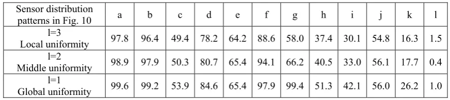
In Table 2, using Eq. (13), uniformity measurement results of omni-directional sensors energy distribution is observed on some samples of node deployments
(a) (b)
Fig. 4. The area covered by sensors to measure the areas energy. (a) Directional sensing area, (b) Omni-directional sensing area (or potential coverage area of
the directional sensor with rotational capability)
Table 2. Uniformity criterion of omni-directional sensors energy for several samples of node deployments
Sensor distribution
patterns in Fig. 10 a b c d e f g h i j k l
l=3
Local uniformity 97.8 96.4 49.4 78.2 64.2 88.6 58.0 37.4 30.1 54.8 16.3 1.5 l=2
Middle uniformity 98.9 97.9 50.3 80.7 65.4 94.1 66.2 40.5 33.0 56.1 17.7 0.4 l=1
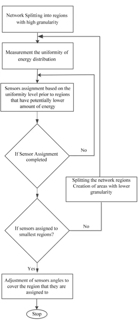
In this secti presented to to maximize network is i presumed t changing it calculated w could poten energy. The entire regio to be divide result, it can in the netw regions can The sta
1. Networ
2. Measur
algorith of this m potentia
3. Sensors
initially
4. Repetiti
to the n
5. Splitting 6. Repetiti sub-reg 7. Adjustm Fig. 5. SE
ion, using an o adjust the s
e the energy initially divi that sensors ts angle of v with respect ntially cover en, it is repea
ns. These sta ed into small
n be expecte work. Based be observed ages of the p
rk Splitting in rement of th hm in the sec model for th ally coverabl s assignment y assigned to ion of stage number of sen
g the networ ion of stage gions. The rep
ment of senso
. 5. Uniformit distributi ENSORS AS S n algorithm sensors angle distribution ided into reg
are directio view. In the to omni-dire . The sensor ated for the r ages can be ler ones, and ed that the un on the Fig. d.
roposed algo
nto large reg he uniformit ction 4, with he sensor wou
le by that sen t based on t regions that 3 until all th nsors. rk regions: th
2 to 5 for ea petition time ors angles to
y criterion of ion patterns fr
SSIGNMEN SENSORS D
presented fo e of view an
uniformity i gions with th
nal, also, ea proposed a ectional mod r assignment
egions with repeated aga d then, senso
niformity of 6, the flowc
orithm are as
ions with the ty of energy the consider uld enable u nsor.
the uniformi t potentially h
e sensors are
he creation of ach of the new es are equal t
cover the re
omni-directio rom Fig. 10 (a
NT TO THE DIRECTION
or the unifor nd the sensor
in a network he highest gr ach sensor c algorithm, th
del for a sen t is initiated the higher en ain for a leve ors assignmen energy distr chart of the
s follows:
e high granu y distributio ration of om us to calculat
ity level and have the low e assigned to
f areas with w regions an to the numbe egion that the
onal sensors en according to T
E NETWOR N ADJUSTM
rmity calcula rs assignmen k with directi anularity. At can choose he uniformity nsor. It speci
from the re nergy until a el with the l nt should be ribution wou sensor assig
larity on in variou mni-directiona e each senso
d energy am wer amount o o all the regio
lower granul nd re-assignm er of granular
ey are assign
nergy of senso able 2)
K REGION MENT
ation in the t to various r onal sensors t first, based its coverage y of energy ifies the regi
gion that ha ll the sensor ower granula
repeated in ld be provid gnment algo
us levels bas al model for or’s energy fo
mount of eac f energy. ons. The repe
larity ment of each
rity levels. ned to.
or
NS VIA
network, a m regions. It is s. For this pu d on the Fig.
e area via ro distribution ions that eve as the lowest rs are assigne arity. Each r smaller regi ded for differ orithm to the
sed on the sensor. Con for the region
ch region: se
etition times
region's sen
method is s provided urpose, the 4(a), it is otation or n is firstly ery sensor t potential ed into the region has ions. As a rent levels e network
presented nsideration ns that are
ensors are
are equal
A novel approach to measuring node and…
June 2013 IJST, Transactions of Electrical Engineering, Volume 37, Number E1
27
According to Fig. 6, the flowchart of the algorithm is shown. In Fig. 7, an instance of algorithm application can be observed. In Fig. 7a, the initial coverage and in Fig. 7b, the coverage after the sensor assignment to the network regions and adjustment of sensors angle of view can be seen. In the following, the simulation results and performance evaluation of the presented methods will be studied.
Fig. 6. Algorithm flowchart of sensor assignment to the network regions
6. SIMULATION AND PERFORMANCE EVALUATION
levels. Glob 8×8 regions is assumed algorithm, t for each pat repetitions) The re Table 1 and has the min the results acceptable r in the low l comparison calculated r intuitively s For exampl indicates the In Tab the algorith the patterns significant a Added regions is a purpose, the regions has of the senso coverage ra by a value o and in the m
bal, middle a s, respectivel equal. The v the value wil ttern, a trial
will be prov esults of unif d Fig. 2. It ca nimum unifo of the unifo range of unif level and the n to Fig. 10g
results from seen that the e, uniformity eir weakness le 3 and Fig. hm applicatio s of Fig. 10 i
and in the ma
7. Sen
d to the unifo another crite e proportion
been measu or assignmen ate of the netw
of coverage i most appropr
and local unif ly. The senso value of φ is ll be calculat set of 10 rep vided as the r formity mea an be seen th rmity. With ormity calcu formity in al e global unifo
g. This is p m the other e two criteria y value for F s.
. 8, the level on for the sen
s shown. It c aximum case
nsor assignatio (b) Angle ad
ormity of en erion that ca n of regions ( ured as the co
nt algorithm work region improvemen riate conditio
formity, in w ors constant s random in ted. Accordi petitions is ge
result. surement of at Fig. 10a h study of the ulation, it is
l three levels ormity is in t proven throu
works ment a lead to the Fig. 10l is sim
of the unifor nsor assignm can be seen t e, it has been
on to region. ( djustment to in
nergy distribu an be utilize (that have be overage rate m to the netw
s before and nt. In the who ons, it is obta
which the net parameters the beginnin ing to the Fig
enerated, als
f the sensor d has the maxim
e other panel shown that s. For instan the high leve ugh the perc
tioned in Eq same result milar to Fig.
rmity of ene ment. Additio
that in the en n 47%.
(a) The initial ncrease the re
ution in the ed for perfo een covered e. In Fig. 7, a work regions d after the sen
ole states, th ained up to 32
twork area ha are R1=5،R2 ng. After app g. 10 the Sen so the averag
distribution mum uniform ls of this figu t the presen
ce, in Fig. 10 el. Figure 10 ceived result
q. (2) and E as the local . 10a, and sh
rgy distribut onally, the im ntire states, t
direction of s gions energy
network, th ormance of by at least o a sample of r s can be obs
nsor assignm e coverage im 2%.
as been split
2=300 ،b=3 plication of t nsor distribu ge value of o
in the netwo mity in all thr ure, and num ted criterion 0f and 10g, t 0f has higher ts as well. I Eq. (3) are l uniformity hows maximu
tion is repres mprovement the level of im
ensors is rand uniformity
e coverage e the proposed one sensor) t
real coverag erved. In Ta ment algorithm
mprovement
t into the 2×2 30˚. Energy o the sensor as ution is perfo outputs (obta
ork are repre ree levels an merical comp n can demon the local uni r middle unif In addition, compared. measuremen mum uniformi
sented before t rate of unif improvement
dom.
extent of the d algorithm to the total n ge with the ap
able 4 and F m have been t is again con
2, 4×4,and of sensors ssignment ormed and ained from esented in nd Fig. 10l
parison of nstrate an
formity is formity in the other It can be nt criteria.
ity, which
e and after formity on t has been
Fig.
Un
L
M
G
June 2013
niformity pat
Local Af im
Middle Af im
Global Af im Distribu patterns in Initi deploym After assi improvem
Table 3. Th
Distribution tterns in Fig.1
Initial deployment fter assignmen mprovement% Initial deployment fter assignmen mprovement% Initial deployment fter assignmen mprovement% Fig. 8. Table 4. ution n Fig.10 a ial
ment 82 gnment 89 ment % 8.
Fig. 9.
A
he uniformity sensor assig
10 a 70.2 7 nt 83.3 8 % 18.6 2 79.5 8 nt 86.0 9 % 8.2 1 89.0 9 nt 94.6 9 % 6.3 0
. Local uniform to
. Coverage rat alg
a b
.4 79.8 .4 93.3 9 5 16.9 3
Coverage rate algo 0.0 20.0 40.0 60.0 80.0 100.0 0 20 40 60 80 100 a
A novel approac
I
y of energy dis gnment algorit
b c
1.4 60.5 8.5 89.2 4.0 47.2 0.2 64.7 2.1 92.9 4.9 43.5 4.1 72.3 4.3 96.8 0.2 33.9
mity of direct o the region (lo
te of the netwo orithm by valu
c d
74 79.3 97.4 95.5 31.6 20.4
e of the netwo orithm by valu
a b c
b c d
ch to measurin
IJST, Transact
stribution leve thm, by unifor
d e
66.9 59.4 88.3 83.9 32.0 41.2 74.4 65.6 93.0 88.2 24.9 34.5 87.7 73.1 96.7 90.7 10.3 24.0
tional sensors ocal uniformit
ork regions be lue of coverag
e f
70.9 79. 93.8 95. 32.3 20.
ork regions bef ue of coverag
d e f g
e f g
ng node and…
tions of Electric
el before and a rmity improve
f g
4 68.0 64 9 86.8 86 2 27.6 35 6 76.6 70 2 91.0 90 5 18.7 27 90.2 85 7 94.1 92 0 4.4 8
energy after s ty in Table 3)
efore and after ge improvemen
g
6 81.1 7 5 92.6 9 0 14.2 1
fore and after e improvemen
h i j k
Init
h i j
cal Engineering
after applicatio ement rate
g h
4.0 58.0 6.5 80.0 5.1 37.9 0.5 62.0 0.0 85.0 7.6 37.0 5.2 67.7 2.4 89.0
.5 31.6
sensor assignm
r sensor assign nt
h i
77.2 69 91.5 86.5 18.5 25.4 sensor assign nt l
tial…
k l Initial…g, Volume 37,
on of the
i j
56.9 60.0 79.7 77.4 40.0 29.0 62.3 66.5 82.8 81.1 33.0 22.0 69.6 72.2 87.5 85.1 25.6 17.8
ment
nment
j k
73.6 62.8 88.5 72.8 20.2 15.9
nment
Number E1
29
k l
53.6 9.2 61.5 9.2 14.7 0.3 57.1 9.0 65.0 9.9 13.8 9.8 67.0 6.0 69.5 6.1 3.8 2.0
l
In this artic This criterio regions to th this criterio network. Al through sen sensor node
Fi
cle, a new cr on can calcu he local unif on was gener
lso, a method nsors assignm es. In order to
ig. 10. A set o
riterion for t ulate the un formity with
ralized for c d was propo ment to the o assess the p
of sensor distri
7.
the uniformi iformity in v
the small re calculation o sed that incr network reg performance
ibution trial pa
CONCLUS
ity measurem various leve egions (aroun of the unifor reased the un gions via ro e of this crite
atterns in the n
SION
ment of the s els from the nd the nodes rmity of the niformity of otating and c erion and the
network [22]
sensor distrib global unifo sensing radi sensor ener energy distri changing of proposed m
bution was p formity with ius). In the n rgy distributi ibution in th
the angle o methods, a set
A novel approach to measuring node and…
June 2013 IJST, Transactions of Electrical Engineering, Volume 37, Number E1
31
distribution patterns was utilized in the network. The gained results represent that the proposed criterion for the uniformity measurement is properly able to measure the local, middle, and global uniformity on the sensor distribution patterns. Moreover, applying this method for the sensor assignment, the uniformity of energy distribution of the network, and the network regions coverage has been extensively increased. In future works, the proposed method can be altered in such a way that sensors are assigned with respect to the network requirements, including targets distribution density in the network regions. Additionally, the distribution of nodes in the network area can be researched in the future works based on the acceptable level of the uniformity of the node. According to the numbers of the covered nodes in the network, the sensor distribution and describing the relation between application types can be found as well. Solving the region assignment to targets after the sensor assignment is another useful study. The parameters of target model such as: size, direction, speed, and other mobility of targets, can affect region assignment strategies.
REFERENCES
1. Tao, D., Ma, H. & Liu, L. (2006). Coverage-enhancing algorithm for directional sensor networks. Mobile Ad-hoc and Sensor Networks, pp. 256-267.
2. Meguerdichian1, S., Koushanfar, F., Potkonjak, M. & Srivastava, M. B. (2001). Coverage problems in wireless ad-hoc sensor networks. IEEE INFOCOM.
3. Chalechale, A. & Safaei, F. (2008). Visual-based interface using hand gesture recognition and object tracking. Iranian Journal of Science And Technology, Transation B, Engineering, Vol. 32, p. 279.
4. Osais,Y., Hilaire, M. S. & Yu, F. R. (2009). On sensor placement for directional wireless sensor networks. Communications Society subject matter experts for publication in the IEEE ICC 2009 proceedings.
5. Jiao, L., Wu, Y., Wu, G., Chang, E. Y. & Wang, Y. F. (2004). Anatomy of a multicamera video surveillance system. Multimedia systems, Springer, Vol. 10, No. 2, pp. 144-163.
6. Heo, N. & Varshney, P. K. (2003). A distributed self spreading algorithm for mobile wireless sensor networks. Wireless Communications and Networking, WCNC.
7. Yuan, L.Y., Yuan, L.Y., Wang, Y. & Luo, W. (2008). Optimized coverage algorithm in WSN based on energy balance. ICCS 2008, Vol. 34, No. 15, pp. 100-101.
8. Bouabdallah, F., Bouabdallah, N. & Boutaba, R. (2009). On balancing energy consumption in wireless sensor networks. IEEE Transactions on Vehicular Technology, Vol. 58, No. 6, pp. 2909-2924.
9. Chang, C. Y., Hung, L. L., Chen, Y. C. & Li, M. H. (2009). On-supporting energy balanced k-barrier coverage in wireless sensor networks. IWCMC '09 Proceedings of the International Conference on Wireless Communications and Mobile Computing.
10. Zhao, E, Zhang, W., Zhang, Q. & Liu, W. (2008). Energy-balanced variable transmission range adjustment in WSNs with quality coverage. 4th International Conference on Wireless Communications, Networking and Mobile Computing, WiCOM '08.
11. Lee, H., Keshavarzian, A. & Aghajan, H. (2010). Near-lifetime-optimal data collection in wireless sensor networks via spatio-temporal load balancing. ACM Transactions on Sensor Networks (TOSN), Vol. 6., No. 3, p. 26.
12. Chang, R. S. & Wang, S. H. (2008). Self-deployment by density control in sensor networks. IEEE Transactions on Vehicular Technology, Vol. 57, No. 3, pp. 1745-1755.
13. Huang, C. F. & Tseng, C. (2003). The coverage problem in a wireless sensor network. Proceedings of ACM WSNA.
15. Wang, D. & Qi, X. (2009). An estimation approach for uniformity of node-distribution in wireless sensor networks. Proceedings of the 5th International Conference on Wireless communications, networking and mobile computing, IEEE.
16. Pescaru, D., Gui, V., Toma, C. & Fuiorea, D. (2007). Analysis of post-deployment sensing coverage for video wireless sensor networks. Proceedings of 6th International Conference RoEduNet.
17. Adriaens, J. (2006). Optimal worst-case coverage of directional field-of-view sensor networks. Communications Society, pp. 336-345.
18. Hussain, S. & Gaudette, L. M. (2006). Quality of coverage of a wireless sensor network using energy efficient routing with genetic algorithms. Sixth International Conference on Recent Advances in Soft Computing (RASC). 19. Hu, T. (2011). Statistical test for multi-dimensional uniformity. M.S. thesis, Florida International University. 20. Guvensan, M. A. & Yavuz, A. G. (2011). On coverage issues in directional sensor networks: A survey. Ad Hoc
Networks, Vol. 9, No. 7, pp. 1238-1255.
21. Hosseini, M., Dehghan, M. & Pedram, H. (2011). Sensor selection using circular target model in Visual Sensor Networks. IEEE International Symposium on Computer Networks and Distributed Systems.
22. Hosseini, M., Dehghan, M. & Pedram, H. (2012). A new measurement method of the node and energy distribution uniformity in the Sensor Networks. 8th International Conference on Information Science and Digital Content Technology (ICIS2101).
APPENDIX 1. THE CALCULATION METHOD OF UNIFORMITY FUNCTION
In order to innovate a suitable uniformity function, assume the following scenario. We assume that the network area is split into N region, also the total number of available nodes in the network is Ns. All the nodes are equally distributed in only y regions out of the total number of regions, y=1 reflects the most non-uniform type of distribution, in which all the nodes are located in one region. y=N is the most uniform type of distribution, in which all the nodes are equally split.
otherwise y i y N Nsi s
, 0
,
where Nsi ,1≤i≤N is the number of available nodes in each region.
In this case, y value can be considered as the distribution uniformity criterion. The objective is to find a linear and an ascending function that provides zero and one (100% uniformity) for y=1 and y=N, respectively. This function is applied for the uniformity measurement in other conditions of node distribution in the network like the sensors distribution pattern shown in the Fig. 10. For this purpose, the node distribution variance based on the y is our starting point:
N y N
Ns y Ns N y Ns y N Ns N Ns N y i N i i 1 1 1 1 1 1 1 ) var( 2 2 2 1 2 1 ) 1 ( ) var( 2 y N N N Ns y
Precise consideration of the variance function would explain why the function is non-linear and unable to appropriately differentiate the uniformity in different cases. Therefore, it is advised to apply a function of var(y) to make it linear. A simple form of this function is the reverse function of var(y).
A novel approach to measuring node and…
June 2013 IJST, Transactions of Electrical Engineering, Volume 37, Number E1
33
As far as the minimum and maximum value of y is 1 and N, respectively, in order to locate the uniformity function between zero and one, we apply a linear equation as shown below:
1 1 1 ) var( 1 1 1 1 1 ) var( 1 1 1 1 1 2 2 N N N y N N u N N y N N N N y u s s
This is equation (3) addressed above. A brief study shows that this function’s value for the completely uniform distribution (var(y)=0) is equal to u=1 and for the entirely non-uniform distribution (var(y)=Ns2 / N) , the function value is zero.
In this regard, the U value for the two boundary states of fully uniform and non-uniform node distribution is as follows:
Fully uniform node distribution: in this case, the number of nodes in each region is equal to the average amount of nodes. Thus, var(NSi) is zero and U is equal to 1 (i.e. 100% uniformity is achieved).
Fully non-uniform node distribution: the most non-uniform type of distribution refers to a case that all the nodes are positioned in the only one region (e.g. the jth region). In this case, the following are true:
otherwise j i N Ns s i , 0 ,
N Ns y Ns N Ns N Ns N Ns Ny N i
i i 2 2 2 1 2 1 1 1 1 ) var(
1 0
1 ) 1 ) 1 (( 1 1 1 1 1 1 1 1 1 1 1 1 1 1 1 ) var( 1 1 2 2 2
2
N N N N N N N N N N N N N Ns N N N N N Ns N N u s i s
Therefore, in Eq. (3), the minimum value of the uniformity variable is zero for the fully non-uniform distribution and its maximum value is equal to 1 for the fully uniform distribution. The variations of uniformity are linear in values in between.