Target tracking solution for multi-sensor data fusion in wireless sensor networks

63

Target Tracking Solution for Multi-Sensor Data Fusion

in Wireless Sensor Networks

Duong Viet Huy

, Nguyen Dinh Viet

University of Engineering and Technology, VNU Hanoi, Vietnam

Abstract

Wireless sensor networks are often composed of many sensor nodes, they are powered by batteries with limited capacity. The sensor nodes are randomly scattered within in the ranger monitoring and send – receiver data using radio waves. Many research projects had demonstrated the consumption of battery power by the data transceiver occupy large compared to the calculation on the sensor node. In this paper, we propose energy saving solutions of nodes in a cluster by only choosing some nodes in the cluster to track the target and transmit this data to cluster head nodes. We based on the location of the sensor nodes in the cluster compare with the location of target and cluster head nodes to perform this selection. The effectiveness of the proposed solutions will be evaluated based on the number of sensor nodes are selected considering the number of nodes in the cluster, this is the base for the effectiveness of energy saving as well as the cluster nodes.

Received 05 December 2015, revised 29 February 2016, accepted 11 March 2016

Keywords: Target tracking, Multi-Sensor Data Fusion, WSNs, ETR-DF.

1. Introduction*

Currently, the monitoring system with sensor networks are developed in size (number of sensor nodes, range monitoring) and quality (parameter monitoring, the fineness of the measurement, etc..). There are different types wireless sensor networks (WSN) architecture to be studied as [1]: flat network, cluster-based

network, tree-based network, grid-based

network, structure free. WSNs with cluster-based network is chosen by many authors to study solutions to save energy. Clustering solutions, typically is algorithms LEACH (Low Energy Adaptive Clustering Hierarchy) at work [2] with the objective of sensor network split into grassroots networks called clusters, communication in clusters in style singlehop or multihop. Each cluster has one cluster head

________

☆_{This work is dedicated to the 20th Anniversary of the IT}

Faculty of VNU-UET

*

Corresponding author. E-mail: [email protected]

(CH) is responsible for data fusion from all of number of sensor node in cluster, while participating in the routing to sending the results of data fusion to the base station (BS). Without loss of generality, we view that a cluster of sensor is a miniature sensor network. And, the content of the article will be directed to the sensor node cluster. With synthesizing data from multiple sensors is "data fusion" or "data aggregation", we will use the term “data fusion”.

When WSNs operates in round, the sensor nodes in the cluster tracking target then sends the data to CH, CH data fusion and send this result to the BS. After each round, the network devide into the new clusters and elect new CH to continue operating. Thus, in each round, all nodes in a cluster must be monitored for 01 target and send the results to CH for data fusion, this has the following challenges: first,

sensor nodes send this the same data on CH will cause redundant data at the CH; secondly, the sending and receiving this redundant data on the network is causes wasting of residual energy of sensor nodes; thirdly, it will cause the risk of network congestion. According to [3], studies [4, 5, 6], energy consumption for the transceiver radio signals many times greater than the energy consumed to process other operations, including the calculation on the sensor node. We will back this content in the following section.

To resolve these challenges, we propose solutions ETR-DF (Efficiency in TRacking to target in multi-sensor Data Fusion in WSNs). The goal of this solution is energy saving of sensor node of the cluster by the optimizing in selecting sensor nodes in the cluster to track the target. The selection was based on the relative distance between the sensor node and the target should be monitored. Effective energy savings expressed in reducing the number of packets must send-receive between sensor nodes in clusters with CH and reduce the amount of data that must be proccess in the CH when CH fusion data. Beside the introduction and conclusion, the content of this article includes 3 main parts: Analysis of the strategic monitoring target of sensor nodes by radio waves; propose solutions ETR-DF; analyse effectiveness of solutions proposed by software simulation.

2. Strategy Of Tracking target

2.1.Target tracking methods

For wireless sensor networks, there are two target tracking methods [7]: target oriented and track oriented. Target oriented is often used when the target is known in advance. The results of target tracking sensor nodes are used to synthesize and make decisions about targets. With track oriented, independent measurements of each node will be determined based on the history of sensor nodes measure that during the

period from start to finish with the measured values in a specified threshold before. This paper uses multi-sensor nodes to monitor a target, there are 3 models tracking Fig.1 [7]:

a) Complementary type

This tracking type in Fig. 1a, the sensor nodes are not directly dependent each other, each sensor node monitoring part of the target, measuring results can be different but they are measurement events of the target. Thus, the measured value of the sensor nodes can be complemented to each other. Inputs to data fusion from the sensor nodes can be better.

b) Competitive type

This tracking types in Fig. 1b, each sensor node independently measure all properties of the entire target. Fusion data from multiple measurement results of sensor nodes on the same set of attributes of the target, the measurement results can be different depending on the time sensitivity of the sensor nodes to the target at the same measuring time or at different time points measured. This tracking type, the CH can tolerance better because CH can compare measurement results of sensor nodes in the data fusion process.

c) Cooperative type

Examples of this type of tracking in Fig. 1c of 2 sensor nodes measuring by image of the target. A sensor node can not measure all the target, CH uses additional measurement results (the intersection) of an other sensor nodes.

2.2. Sending - receiving data by radio wave

Energy consumed on each sensor node in Fig. 2, there are 03 Units of energy consumption [8]:

Processing unit (PU): Consumption of energy to control and process entire operation of the sensor node. PU includes data storage and CPU processing.

Sensing unit (SU): Consumption of energy to provide sensing and transmission of information about the event of the target to PU.

SU includes sensor, adapter A/D

(analog/digital) signal conversion Digital to Analog (from PU to SU) and signal conversion Analog to Digital (from SU to PU).

Communication unit: Power consumption to communicate signal as sending data or receiving data by electromagnetic waves from the sensor node to another node or BS.

According to the statistics [2], the energy consumed by transceiver radio signals many times greater than the energy consumed to process task other of sensor node, including the calculation on the sensor node. Chart comparing the rate of energy consumption during sensor operation in Fig. 3. The relationship between energy consumption ETX

when sending k bit with distance d and ERX

when receiving k bits have been proven in [1]:

ETX = Eelec*k+Eamp*d2 and ERX=Eelec*k, where

Eelec is energy consumption of sensor node to

send or receiving 1 bit, Eamp is energy

consumption of sensor node to sending 1 bit/m2

by radio signals.

Thus, the energy of the electromagnetic waves transmitted from the sensor node data.

They will decrease exponentially compared to the distance between sender node and receiver node, to ensure the packet to its destination. The sensor node must to manually adjust (amplifier) power transmitters with the square of the distance [1]. For this reason, research groups oriented to reduce the amount of data sent from sensor node.

3. ETR-DF solution

3.1. Input data to fusion

As discussed in Part II, A, target measurement data from the sensor nodes can be same completely or partially. If all the same data are sent to CH by sensor nodes (for synthesis). It will also cause of excess data at CH and the risk of traffic congestion. More importantly, useless energy wasted when sending the same data to CH.

Therefore, in this paper we use the competitive type and target oriented tracking method because the amount of the target be known in advance and the measurement results are cyclical. We aim to select sensor nodes based on the relative position between the sensor nodes and target, sensor node and CH. The target of tracking and resolving partially drawback above is solution named ETR-DF.

3.2. Selecting the sensor node

After being scattered randomly, the sensor nodes will have a fixed location with assuming the BS and the sensor nodes located in plane geometry, and BS have a fixed location. Thus,

Figure 2. Diagram of power supply for sensor node [8]. Power

Communication Unit

Sensor A/D

Storage

CPU Processing

Unit

Sensing Unit

BS is easily to identify the location of the sensor node (BS completely determine the relative position between the sensor nodes in the network and BS). Additionally, the sensor node designed distance measurement function to neighboring sensor nodes received through signal strength indicator (RSSI receive signal strength) or Time of arrival (TOA) ... [12] With this function to sensors node measure the distance, coordinates of sensor node and adjust transmit power to match the distance to receive sensor node.

Suppose there is a cluster of sensor nodes (S) consists of n nodes are scattered randomly on a plane. It’s known that the location of a target (Tag) and a cluster heads node (CH). Initially, the residual energy of sensor nodes are the same. In the process of using the energy of the decline sensor node and the inventory levels can not be equal. ETR-DF solution selects sensor nodes located on the road shortest between CH and Tag. Without loss of generality, in this paper, we use the distance calculation in plane geometry.

a) Selected sensor node area

• Distance

It can be considered sensor nodes, Tag, CH are the points in the plane, then the coordinates of the points are Node (xnode, ynode ), Tag (xtag, ytag ), CH (xCH , yCH ). Call d node-CH , d

node-tag , d CH-tag are respectively distances between sensor nodes and CH, between sensor nodes and Tag, between CH and Tag and they are calculated as follows:

(

) (

)

CH node CH

node CH

node

x

x

y

y

d

=

−

−

−

(

) (

)

tag node tag

node tag

node

x

x

y

y

d

=

−

−

−

(

) (

)

tag CH tag

CH tag

CH

x

x

y

y

d

=

−

−

−

Between CH and Tag always exist one line d0 , straight lines d1 and d2 perpendicular to

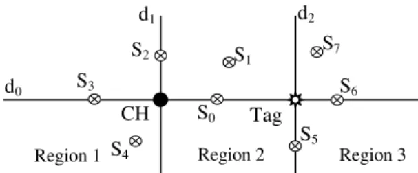
go through CH and Tag. They divided space to sections as Fig. 4. An example, the position of the sensor node S0 to S7 with CH and Tag are

corresponding with 8 probable cases:

We found that if at the time of review, the residual energy of nodes are the same, and measure Tag and send to CH with the same data unit. The nodes located on the straight line connecting CH with Tag (eg sensor node S0 in

Fig. 4) may consume less energy because the distance d = dnode-CH + dnode-tag = d CH-tag = d min.

Sensor node get data from the target and forward this data to the CH. So, the capacity of input data and capacity of output data of sensor node almost the same. In this case, the distance factor will determine the energy consumption. Call Ednode-tag and Ednode-CH are respectively

energy consumption of sensor nodes when measuring target and sending data to CH. Then:

Ednode-CH > Ednode-tag according to [6] and the

case for dnode-CH = dnode-tag. So in this case, the

node S0 near CH may be more efficient in energy saving.

• Deviation of distance

We propose to use the number δ ≥ ₀ to determine the limit of the distance incorrect position of the sensor compared to the boundary determined priority areas, priority levels. δ is used only in blocked areas by d1 and d2. This

means that if a horizontal axis (Ox) contains

d0, the origin O is the midpoint of CH and Tag. We only consider the sensor nodes coordinate axis Ox on blocked area (or close area) [-(d

CH-Tag)/2, (dCH-Tag)/2] Where δ = 0, the sensor nodes

are on the boundary. Since δ≥ 0 and there are 3 priority levels, so a sensor node can belong to many different priority levels. The location of

Figure 4. Position of the sensor node with CH, Tag.

d1 d2

Tag S0

S1

CH

S7

S6

S5

S4

S2

S3

d0

Region 2

sensor nodes are in the intersection area of priority levels.

• Priority area

Based on the analysis of the distance between sensor nodes, CH and Tag, ETR-DF solution focuses on analyzing region 2 - area bounded by d1, d2 and including d1, d2 in Fig.

4. Region 2 is divided into priority areas and priority levels in Fig. 5. The priority level from high to low is used by CH in case of selection

results-measurement of target to data

fusion. This means that, in the same period of cluster activity, the CH can select any node in the cluster sensor of priority areas that have higher priority, using measure results to data fusion. In these priority areas, criteria of selecting sensor nodes of CH, except for the priority levels, there also have other criteria such as energy sensor node reserves, the packet must be forwarded to the CH to complete measurement data target, rate d node- CH/d node-tag, etc.

If the location of sensor nodes from high to low priority are following: Level 1 is a straight line CH-Tag; Level 2 limited by the diameter circle CH-Tag; Level 3 the area bounded by Ellipse have 2 special points CH, Tag and focal (or focal distance) dCH-tag.

The first priority area (A-Prio1) inFig. 5a is rectangular with 2 edges d CH-Tagand 2δ,

coordinates 4 points (-(xCH + xtag)/2, -δ), ((xCH +

xtag )/2, -δ), ((xCH + xtag)/2, δ), (-(xCH + xtag)/2, δ).

The 2nd priority area is annulus that limited by 2 circles (center O) in Fig. 5b, radius R1 =

(dCH-Tag/2) - δ (limited to inner circle) and the

center O, radius R2 = (dCH-Tag/2)+δ (limit outside

the circle). Priority Area for level 2 is annulus and blocked by d1, d2, A-Prio2 = π * [((d CH-Tag /

2) + δ_{)2-((d CH-Tag/2) -} δ_)2] [11].

The 3rd Priority area (A-Prio3) is the area bounded by the ellipse in Fig. 5c. The Ellipse has CH, Tag, called semi-major axis, small axis, haft focal, eccentricity of Ellipse are aellipse ,

bellipse , c ellipse and e ellipse .

Set cellipse = bellipse = dCH-Tag/2

Tag CH ellipse

ellipse c d

b

a = + = −

2 2

2 2

ellipse

and

2 2 ellipse=

e [11]. We set the hypothesis,

there exists at least one sensor node of at least 1 in 3 priority areas.

We set the hypothesis, existing at least one sensor node located in priority areas. Then, the sensor node as sensor node normal role and CH role. Thus, the scope to select the sensor node is union of three priority areas A-Prio1, A-Prio2

and A-Prio3.

Of course, the case of a sensor node in 2 (or 3) the priority areas, then the selection will be based on right balance between the priority area and other attributes of the sensor node as the remaining energy of sensor node, number of packets required to send to CH etc. We will continue to study this problem in the future.

a

l

d1 d2

d0

Level 2 (bounder) x O

Tag CH

δ δ

R0

R1

R2

A-Prio2 d1 d2

d0

Level 3 (bounder) x O

Tag CH

bellipse

A-Prio3

cellipse

aellipse

d1 d2

d0

Level 1 x O

δ

A-Prio1

Tag CH

(a) (b) (c)

b) ETR-DF algorithm

1. Set n = num_cluster_nodes; δ_;

2. Define CH,Tag

and set CH(xCH, yCH),Tag(xtag, ytag);

3. The CH-Tag line in horizontal axis (Ox), yCH = ytag = 0;

4. Origin is midpoint CH-Tag line, O((xCH + xtag)/2, 0);

5. Define d(node,CH), d(node,Tag), d(CH,Tag); 6. Identify priority areas:

A-Prio1, A-Prio2, A-Prio3;

7. Select sensor node in cluster, add nodes to priority areas;

8. For {set i 1} {$i <= $n } {incr i};

9. If not any Si belong to A-PrioJ (j=1, 2, 3)

then add CH to node_prioJ

10. Else Si belong to A-PrioJ (j=1, 2, 3) then

add Si to node_prioJ;

11. Sent data to CH

12. Set m = num_nodes_ prioJ ;

13. For {set j 1} {$i <= $3 } {incr j}; 14. For {set k 1} {$i <= $m } {incr k}; 15. Sent Sk.data_measure to CH;

16. End.

Right after clusters have been established, there have nodes in the cluster and CH, ETR-DF algorithm is started. Line 1, set number of node in cluster and deviation of distance δ. Line

2, Define CH, Tag and determine the

coordinates of CH, target (Tag). Line 3, 4, CH-Tag line on the horizontal axis (Ox), O point is a centre of circle and midpoint of CH-Tag line.

Line 5, determine distance between sensor node and CH, sensor node and target, CH and target.

Line 6, identify priority areas with deviation of distance δ. Line 7 to 10, in priority areas, select sensor node in cluster and belong to priority areas (line 9), add nodes to priority areas (line 10) for selecting sensor node next step. Line 11 to 15, selects sensor node in node_prioJ set with k sensor node, k may variable depend on node priority set, then this sensor node sends data measure about target to CH. Line 16, the end of round.

3.3. Simulation and analysis

a) Parameters simulation

Table 1: The main parameters

Parameter Value

Number of sensor nodes 100 Coordinates node in the (100m x 100m) Random The min and max number of clusters 1 → 10 The number of clusters desired 5 Initial residual energy of sensor nodes 2 J Energy to receive 1 bit 5 nJ Energy consumption to send 1 bit 50 nJ Amplification factor radio transmissions 10pJ/bit/m2 Capacity of node while Idle or Sleep 0 W Speed of radio transmissions 1 Mbps Header size (hdr_size) 25 Byte Sensing data size (sig_size) 500 Byte Time per round/ data fusion (T) 20 s (option) Number of sensor nodes in cluster (n) Random Deviation of distance (δ) 1 m

b) Analysis and evaluation efficiency

We use NS2 simulation software, version 2.34 installed on Ubuntu 12.04 operating system and source code from MIT (Massachusetts Institute of Technology) [2, 9, 10]. The parameters ETR-DF simulation are in Table 1.

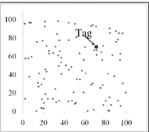
Simulations with 01 Target (70, 70), 100

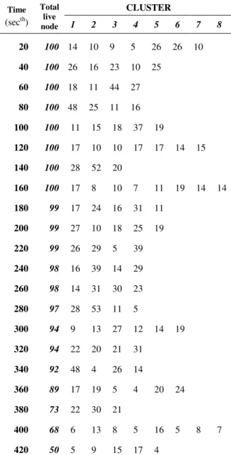
sensor nodes (residual energy 2J/node) are randomly distributed in Fig. 6, network automated clustering with LEACH algorithm [2]. Time per round T = 20s, can change T. At the beginning of each cycle, sensor network including 100 sensor nodes is divided into clusters, the number of sensor nodes in each cluster may be different in Table2.

Figure 6.The position of the sensor nodes in the survey plane.

In each round, we will examine the cluster has the most sensor nodes, apply ETR-DF

algorithm to ensure repeatability and

representation of the sampling size. During the survey, after cycle T = 20s, network clustered again, the number cluster and numbers in each cluster node sensor in Table 2. In each cycle, we use ETR-DF algorithms for sensor node cluster. For example at 80th second, sensor network is divided into 4 clusters in Fig. 7, the nodes in the clusters and CH of cluster following LEACH algorithm, distributed nodes position as follows: Cluster 1: 48 nodes (Fig. 7a), Cluster 2: 25 nodes (Fig. 7b), Cluster 3: 11

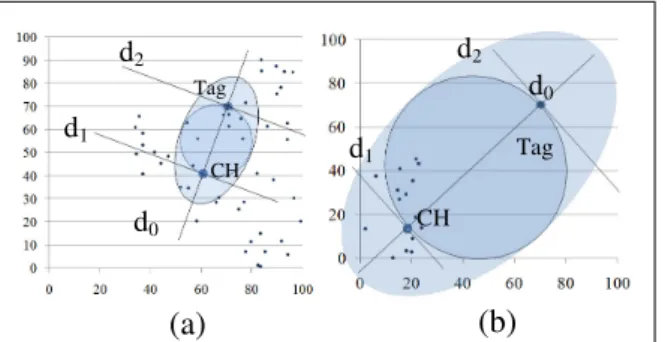
nodes (Fig. 7c), Cluster 4: 16 nodes (Fig. 7d). Applying ETR-DF solution to choice measurement results from the sensor nodes in the cluster, an example for Cluster 1 and Cluster 4 in Fig. 8.

Cluster 1 with 48 sensor nodes (including the CH): after applying the algorithm ETR-DF,

13 of the 47 sensor nodes are selected by CH node to retrieve data. Thus, there are 34 sensor nodes without energy loss due to send data to CH. With simulation profile in Table 1 and the simulation results, we calculate the size of sensing data (sig_size) savings from 34 sensor nodes is 681, equivalent to 681 sig_size * 500

byte/sig_size = 340,500 bytes. Energy

consumption to send 1 bit is 50nJ, so energy savings of 340,500 bytes * 8bit / byte * 50nJ / bit = 136,200,000 nJ = 136,200 µJ = 0.1362 J. In this case, the energy saving efficiency reaches 76.5%.

With Cluster 4, when applying ETR-DF, all nodes participate in send and receive data processes, energy-saving efficiency is 0%.

However, there are some cases that energy-saving efficiency reaches 100%. For example, network is divided into seven clusters at 120th seconds, each cluster node numbers in Table 2. According to the simulation results the position of the nodes of the cluster 7, CH and Tag in Fig.9.

Several experiments have been performed to illustrate the effectiveness of the proposed ROI-BA method. The experiment results are reported for several video sequences using 3D test model (3DTM) reference software [15] of the 3D-HEVC extension of H.265/HEVC standard at 30 frames/s. The four main test sequences used in our experiments are Ballet,

Breakdancers, Alt Moabit, and Book Arrival

with resolution is XGA 1024×768, and each sequence consists of 8/16 color views captured

from different cameras (100 frames per view). Along with color views are correlative depth maps generated from stereo. The former two test sequences come from [16] by Microsoft, while the latters are provided by [17]

from Heinrich Hertz Institute. In our

experiments, the value of α is set to 1.3 for Alt Moabit test sequence and 1.25 for three remaining samples. The first test sequence

Ballet contains a dancing-ballet woman and a watching-man in a room. The second,

Breakdancers, contains a dancing man and four other men are watching him in a practicing room. The third test sequence, Alt Moabit is a traffic scene in Berlin with some cars parked down near the pavement while other cars are moving. The final one is Book Arrival with a man sits in the room before another man coming in and they have a talk.

the BA scheme is performed without considerring the

ROI detection and ROI based BA.The QPs values in [7] therefore are equally assigned to

Figure 7.Cluster and number of node in cluster.

(a) (b)

(c) (d)

Tag

Tag Tag

Tag

Table 2.Number of cluster, sensor

CLUSTER Time

(secth) Total

live

node 1 2 3 4 5 6 7 8

20 100 14 10 9 5 26 26 10 40 100 26 16 23 10 25

60 100 18 11 44 27 80 100 48 25 11 16 100 100 11 15 18 37 19

120 100 17 10 10 17 17 14 15 140 100 28 52 20

160 100 17 8 10 7 11 19 14 14 180 99 17 24 16 31 11

200 99 27 10 18 25 19 220 99 26 29 5 39 240 98 16 39 14 29 260 98 14 31 30 23 280 97 28 53 11 5

300 94 9 13 27 12 14 19 320 94 22 20 21 31

340 92 48 4 26 14

360 89 17 19 5 4 20 24 380 73 22 30 21

Table 3. The average effective fusion of cyclic clusters in simulation between ETR-DF and LEACH

Time (sth) 20 40 60 80 100 120 140 160 180 200 220 ETR-DF 553 730 1175 833 928 1587 1236 377 1228 870 589

LEACH 1328 2638 2125 1725 1709 2074 1893 1286 3076 2308 2116

Efficent (%) 41.64 27.67 55.29 48.29 54.30 76.52 65.29 29.32 39.92 37.69 27.84

Time (sth) 240 260 280 300 320 340 360 380 400 420 ETR-DF 1152 902 752 547 1193 950 722 569 204 747

LEACH 1590 1714 1719 1303 2683 1716 1082 1790 868 1644

Efficent (%) 72.45 52.63 43.75 41.98 44.47 55.36 66.73 31.79 23.50 45.44 Figure 8.Apply ETR-DF to select sensor node,

Cluster 1 with 48-nodes in figure 8a and Cluster 4 with 16-nodes in figure 8b.

d1

d2

d0

d2

d1

d0

Tag CH

CH Tag

(a) (b)

Figure 10. Comparing the number of packets to transmit by ETR-DF and LEACH.

This is a special case when applying ETR-DF because CH plays two roles as a sensor node and a CH node. Effect of energy savings of clusters reaches 100%. However, in this case, conditions are CH node must be dependable and using measure results from a sensor node does not affect to the measure efficiency. We expect to continue to research this problem in the future.

By analyzing data for all clusters in each cycle T = 20s and comparing with LEACH algorithm in the simulation time to the 420th

second, we can realize that nodes rate selected with total nodes in clusters with about great oscillations, from 0% to 100% in each cluster. However, if calculating in each cycle the T the effection is between 23.5% and 76.52%. The average effective fusion of cyclic clusters in simulation time of cycle T between ETR-DF and LEACH in Table 3. Effective energy saving by limiting the data sent by radio waves in Fig.10.

4. Conclusion

We have proposed the solution of cluster target tracking sensor nodes based on the distance between the sensor nodes with CH and target in this paper. This solution has effect to reduce the amount of data to synthesize CH input data by reducing the number of packets to be transmitted from the sensor nodes in the cluster send to CH, so it saves enegry of sensor nodes simultaneously, limits the risk of causing congestion.

ETR-DF algorithm efficiency will be better if the residual energy of sensor nodes is relatively uniform, then the distance is the main criterion for choosing the sensor node. In addition, the measurement reliability of the sensor node is being considered because in some cases, measurement data from a sensor node may be better than the aggregated results from multiple sensor nodes. This is very natural for data fusion from multiple sensor in wireless sensor networks.

In the future, we will research the optimal solution in choosing the sensor nodes based on remain energy of sensor nodes and location of the sensor node to the position of CH and target. We will also research special case when

applying ETR-DF with cases exist only CH in the priority region.

References

[1] Vaibhav Pandey, Amarjeet Kaur and Narottam Chand, “A review on data aggregation techniques in wireless sensor network”, Journal of Electronic and Electrical Engineering, Vol. 1, Issue 2, 2010, pp.01-08.

[2] W. Heinzelman, A.P. Chandrakasan and H. Balakrishnan,“Energy-Efficient Communication Protocol for Wireless Microsensor Networks”, IEEE Proceedings of the Hawaii International Conference on System Sciences, January 4-7, 2000, Maui, Hawaii.

[3] Kazem Sohraby, Daniel Minoli, Taieb Znati,

“Wireless Microsensor Networks Technology,

Protocols, and Applications”, Published by

John Wiley & Sons, Inc., Hoboken, New Jersey, 2007, pp. 307-319.

[4] W. Heinzelman, A. Chandrakasan, H. Balakrishnan, ‘‘An Application-Specific Protocol Architecture for Wireless Microsensor Networks,’’ IEEE Transactions on Wireless Communications, Vol. 1, No. 4, Oct. 2002, pp. 660-670.

[5] A. A. Ahmed, H. Shi, Y. Shang, ‘‘A Survey on Network Protocols for Wireless Sensor Networks’’, Proceedings of Information Technology Research and Education (ITRE), 2003.

[6] C. Schurgers, V. Tsiatsis, S. Ganerival, M. Srivastava, ‘‘Optimizing Sensor Networks in Energy-Latency-Density Design Space’’, IEEE Transactions on Mobile Computing, January 2002, pp. 70-80.

[7] Jitendra R. Raol, “Multi-Sensor Data Fusion with Matlab”, CRC Press, by Taylor and Francis Group, 2010, pp 97-206.

[8] Bing Liang, Qun Liu, “A Data Fusion Approach for Power Saving in Wireless Sensor Networks”, Proceedings of the First International Multi-Symposiums on Computer and Computational Sciences (IMSCCS'06 - 2006), Vol 2, pp. 582 - 586. [9] Network Simulator: http://isi.edu/nsnam/ns/ [10]Neha Singh, Prof. Rajeshwar Lal Dua, Vinita

Mathur, "Network Simulator NS2-2.35", International Journal of Advanced Research in Computer Science and Software Engineering, Volume 2, Issue 5, May 2012.

[11]https://en.wikipedia.org/wiki/Annulus_(mathematics) https://en.wikipedia.org/wiki/Ellipse