JIEM, 2018 – 11(4): 749-768 – Online ISSN: 2013-0953 – Print ISSN: 2013-8423 https://doi.org/10.3926/jiem.2649
A Condition-Based Opportunistic Maintenance Policy Integrated with
Energy Efficiency for Two-Component Parallel Systems
Aiping Jiang , Yuanyuan Wang , Yide Cheng
Sydney Institute of Language and Commerce, Shanghai University (China)
[email protected], [email protected], [email protected]
Received: May 2018 Accepted: September 2018
Abstract:
Purpose: This paper deals with the problem of traditional maintenance model ignoring energy consumption in two-component parallel systems. Thus, the aim of the article is to propose a new maintenance model with ecological consciousness for two-component parallel systems, which can improve the energy utilization and achieve sustainable development. The objective is to obtain the optimal maintenance policy by minimizing total cost.
Design/methodology/approach: This paper integrates energy efficiency into condition-based maintenance (CBM) decision-making for two-component parallel systems. Based on energy efficiency, the paper considers the economic dependence between the two components to take opportunistic maintenance. Specifically, the objective function consists of traditional maintenance cost and energy cost incurred by energy consumption of components. In order to assess the performance of the proposed new maintenance policy, the paper uses Monte-Carlo method to evaluate the total cost and find the optimal maintenance policy.
Findings: Simulation results indicate that the new maintenance policy is superior to the classical condition-based opportunistic maintenance policy in terms of total costs.
Originality/value: For two-component parallel systems, previous researches usually simply establish a condition-based opportunistic maintenance model based on real deterioration data, but ignore energy consumption, energy efficiency (EE) and their contributions of sustainable development. This paper creatively takes energy efficiency into condition-based maintenance (CBM) decision-making process, and proposes a new condition-based opportunistic maintenance policy by using energy efficiency indicator (EEI).
Keywords: energy efficiency, condition-based opportunistic maintenance, two-component parallel systems
To cite this article:
1. Introduction
For fear of sudden failure, most companies are willing to repair/replace their components before breakdown. Garg, Rani, and Sharma (2013) simultaneously consider mechanical service, repair and replacement in periodic preventive maintenance. However, this maintenance policy only focuses on the fixed preventive maintenance interval, but ignore the real deterioration level of components. Nowadays, condition-based maintenance is used extensively in various industries, and companies always regard this method highly to ensure maintenance before breakdown. Although the corporations give high priority to the periodic preventive maintenance or condition-based maintenance, they ignore the fact that maintenance activities can strengthen or weaken the ecological burden exerted by system. Horenbeek, Kellens, Pintelon, and Duflou (2014) points out that energy, resources and environment all belong to the category of ecology. It came to be a common situation that companies take blind eyes to the machines in bad condition, since they will not maintain the components when they can still work, even if these components are gradually in poor state which will increase energy consumption. For instance, a ship company, when encounters motor boilers, blowers, belt conveyor belt relaxation and induced draft fan adjustment door open and closed out of work, will not conduct instant maintenance for the purpose of saving money, if these devices mentioned above incur small problems but they can still on operation. However, the negative point is that continuous uses without maintenance will seriously affect the key indicators alpha value of the combustion conditions (ie, air excess coefficient). In general, when the value is too large, the fan energy consumption increased sharply.
With the enhanced awareness of energy conservation, a new trend concerning about saving energy, protecting the environment, and achieving sustainable development is prevalent in modern society. In actual industrial production, a great amount of energy, such as electricity, etc. needs to be consumed to maintain machines’ normal operation, and if the system cannot work in good condition, there would be much more energy loss in the manufacture process and thus pose a huge burden on the whole ecology. Thus, for most of the enterprises, it should be the long-term strategic focus how they can apply valid maintenance activities to the improvement of system's resource utilization and establishment of a green image. Traditional maintenance mainly focuses on controlling maintenance fee at a low level and keeping the reliability of the system at a high level, but ignores to avoid excessive energy consumption under operation. Therefore, it is imperative to consider the energy consumption of system under operation when developing a maintenance policy.
The rest of the paper is structured as follows: In section 2, several related research literatures are reviewed. Section 3 presents degradation model of individual component and introduces the energy efficiency indicator. Section 4 proposes the new condition-based opportunistic maintenance policy integrated with energy efficiency (EE). Section 5 conducts numerical experiments to testify the advantage of new proposed policy by comparing new proposed and classical maintenance policy. Finally, conclusions and future work are stated in Section 6.
2. Literature Review
The economic dependence provides opportunities to maintain several components jointly, and thus reducing high fixed set-up costs (such as sending a maintenance team to the site, which incurred once maintenance action is performed on one component). Several literatures have pointed out that group maintenance actions can reduce the total costs of the system (Bouvard, Artus, Bérenguer, & Cocquempot, 2011; Qian & Wu, 2014; Tian, Jin, Wu, & Ding, 2011; Tian & Liao, 2011; Zhang, Zhou, Sun, & Ma, 2012). When considering economic dependence, it is sensible to take group or opportunistic maintenance policies into account. Opportunistic maintenance can be recognized as dynamic group maintenance, because workers will not maintain non-failed components unless they are in opportunistic zone (Cavalcante & Lopes, 2014). Compared with group maintenance, opportunistic maintenance can reduce the waste of maintenance resources.
Several papers have proposed opportunistic maintenance policy in CBM in terms of economic dependence. Wijnmalen and Hontelez (1997) is the first one to propose a condition-based opportunistic maintenance policy based on deterioration level of components. It points out that if one component is going to repair, group maintenance actions only occur when the deterioration level of another component is over its opportunistic threshold. Barbera, Schneider, and Watson (1999) proposes a condition-based opportunistic maintenance policy based on exponential failures for a two-component series system. And finally, the long-term average cost is minimized by dynamic programming. When comes to a two-component series system, Castanier, Grall, and Berenguer (2005) also formulates a condition-based opportunistic maintenance policy, in which the deterioration level can be obtained by non-periodic inspections. It points out that the degradation process of the system after maintenance has the semi-regenerative properties and this policy finally establishes a minimum cost rate model based on the semi-renewal theory. For a two-component parallel system, Li, Deloux and Dieulle (2016) studies a condition-based maintenance policy considering both stochastic and economic dependence among components. It presents a new decision rule which permits the maintenance grouping in advance or postponed maintenance. Zhu, Peng, and Houtum (2015) presents an optimal CBM policy that minimizes the long-term mean maintenance cost per unit time for a multi-component system with continuous deterioration. They point out that it is more economical to preventively maintain several components simultaneously. Finally, the advantage of the presented policy is analyzed by a three-component series system of wind turbine. In recent years, some scholars intend to optimally plan maintenance activities for multi-component systems based on prognostic information and presents a dynamic predictive maintenance policy for multi-component systems (Bian & Gebraeel, 2014; Nguyen, Do, & Grall, 2014; Shi & Zeng, 2016). Furthermore, Jiang, Duan, Tian, and Wei (2015) and Keizer, Teunter and Veldman (2016) propose a condition-based opportunistic maintenance policy for redundancy systems separately. Jiang et al. (2015) establishes a reliability analysis model of the system with the basis of the remaining useful life (RUL) of components. This real-time sampling can reduce unnecessary preventive maintenance costs and high fixed maintenance costs of components, thereby increasing the efficiency of the whole redundant system. Finally, three numerical examples are used to verify the feasibility and flexibility of the model. Keizer et al. (2016) points out that in redundancy systems, the maintenance of some failed components can be postponed, under the condition that the reliability of the whole system is not reduced. Finally, the optimal maintenance policy can be obtained by dynamic programming. Despite the single-objective model above, some scholars are inclined to multi-objective optimization. Garg (2016) presents a method for obtaining the optimum maintenance interval by considering maximum availability and minimum maintenance cost. For a series system, Garg and Sharma (2013) consider the maximum reliability of system and minimum design cost as the two objectives. Then, they solve the reliability allocation problem of subsystems by fuzzy nonlinear programming. Based on the two objectives, Garg, Rani, Sharma, and Vishwakarma (2014a) allocate the reliability for a series-parallel system. As well known, reliability and cost parameters are under uncertainties normally in design phases. Therefore, under the condition that parameters are imprecise, Garg, Rani, Sharma, and Vishwakarma (2014b) utilize intuitionistic fuzzy programming techniques to solve a multi-objective reliability optimization problem.
the increasingly serious problems of energy and environment, several literatures of CBM with ecological awareness have been proposed over the past decade. Hoang, Do, and Iung (2016a, 2017) point out that maintenance activities (such as maintenance time, preventive or corrective maintenance, etc) can be influenced when considering some ecological aspects. Mora, Vera, Rocamora, and Abadia (2013) and Xu and Cao (2014) conclude that different maintenance actions on deteriorated components can lead to different effect on ecology. Horenbeek et al. (2014) is the first one to integrate ecological factors in a maintenance optimization model. This model can be considered as an ecological analysis tool which covers many maintenance strategies (such as failure-based, block-based and use-based maintenance). Then, the presented model, which concerns an integrated economy and ecology, can determine the optimum maintenance interval. Chouikhi, Dellagi, and Rezg (2012) propose a CBM model from the respect of probability and statistics and combine environmental problems with maintenance activities. Preventive maintenance takes place when the amount of released refrigerant gas exceeds the alarm threshold and this action helps enterprises avoid a large penalty cost caused by excessive refrigerant gas release. Tlili, Radhoui, and Chelbi (2015) has made a further improvement in 2015. It proposes a preventive maintenance threshold value below the alarm threshold, which can avoid a huge economic penalty more effectively. In addition to the environmental problems (the release of refrigerant gas, etc.), some scholars also consider energy consumption in CBM decision-making. Hoang et al. (2016b) proposes a CBM model for a single-component system considering the energy consumption, in which maintenance activities can be performed based on the energy efficiency (EE) of the components. This model aims to minimize the total cost including maintenance cost and energy consumption cost. Nevertheless, literatures, in which CBM model stresses energy consumption during components’ normal operation for multi-component systems are absent till now. In view of this situation, we propose a new condition-based opportunistic maintenance model integrated with energy efficiency for a two-component parallel system in this paper.
3. Degradation Model and Energy Efficiency Indicator
Throughout this paper, we consider a two-component parallel system. The energy consumption of the system is the sum of energy consumption of individual component. The two components have their own different energy consumption process incurred by different degradation process of them.
3.1. Notations
Some notations used in this paper are summarized as follows: ΔTi: Fixed inspection interval of component i, i = 1,2
Ei(t): The energy consumption during one-time unit of component i (from t to t + 1), i = 1,2
EEIi(t): The energy efficiency indicator during one-time unit of component i, i = 1,2
EEILi: Corrective maintenance threshold for component i in new proposed maintenance policy, i =1,2
EEIMi: Preventive maintenance threshold for component i in new proposed maintenance policy, i = 1,2.
EEIMi < EEILi
Xi(t): Degradation level during one-time unit of component i, i = 1,2
Li: Corrective maintenance threshold for component i in classical maintenance policy, i = 1,2
Mi: Preventive maintenance threshold for component i in classical maintenance policy, i = 1,2. Mi < Li
αi:, βi: Scale and shape parameters of the deterioration process of component i
Si: Running speed of component i, i = 1,2
Oi: The useful output during one-time unit of component i, i = 1,2
ICt: Cumulative inspection cost of the whole system during the period (0, t]
MCt: Cumulative maintenance cost of the whole system during the period (0, t]
ECt: Cumulative energy cost of the whole system during the period (0, t]
CO: Long-run expected cost of system per useful output unit : Each deterioration inspection cost of component i, i = 1,2 : Each energy consumption inspection cost of component i : A preventive maintenance cost for component i, i = 1,2 : A corrective maintenance cost for component i, i = 1,2 cs: A fixed set-up cost
Ep: The energy price
: The number of preventive maintenance for component i, i = 1,2 : The number of corrective maintenance for component i
: The number of inspection for component i : The number of grouping maintenance
: The amount of energy consumption for component i during the period (0, t]
Pp2: The probability that the energy efficiency indicator of component 2 exceeds its preventive maintenance
threshold at current inspection time
Pc1: The probability that the energy efficiency indicator of component 1 exceeds its legislation at the next inspection
time.
PP: The opportunity maintenance threshold in new proposed maintenance policy and it is the threshold of Pp2 PC: The postponed maintenance threshold in new proposed maintenance policy and it is the threshold of Pc1 PP': The opportunity maintenance threshold in classical maintenance policy
PC': The postponed maintenance threshold in classical maintenance policy
CS: The cost saving, it is the difference between CO* of Policy 0 and that of Policy 1
3.2. Degradation Model
The Gamma process has been successfully selected to describe the gradual degradation process of individual component in different industrial systems (Dieulle, Bérenguer, Grall, & Roussignol, 2003; Noortwijk, 2009). The Gamma process has several characteristics as follows:
• Xi(0) = 0, i = 1,2.
• Xi(t) has independent increments,
• For t > τ > 0, the increment of deterioration level for component i Xi(t) – Xi(τ) follows a Gamma
probability density function with the shape parameter αi(t – τ) and the scale parameter βi:
(1)
Given α1 = 1, β1 = 1 and α2 = 1, β2 = 2, then the degradation process of two components are illustrated in Figure
Figure 1 reveals clearly that the deterioration level of each component increases gradually as the time flies. However, the degradation rate of component 1 is lower than that of component 2, because the scale parameter αiβi
represents the degradation speed of component i and α1β1 < α2β2. Generally, different couples of parameters(α and β) can generate different deterioration behaviors.
Figure 1. Degradation process of two components
3.3. Energy Efficiency Indicator
Hoang et al. (2016b) has pointed out that energy consumption of component i varies over time and it depends on the degradation level and the running speed. In order to ensure the stable operation of the whole system, we need to control the running speed of different components (constants in this paper). Therefore, the energy consumption during one-time unit depends only on the deterioration level X(t):
(2)
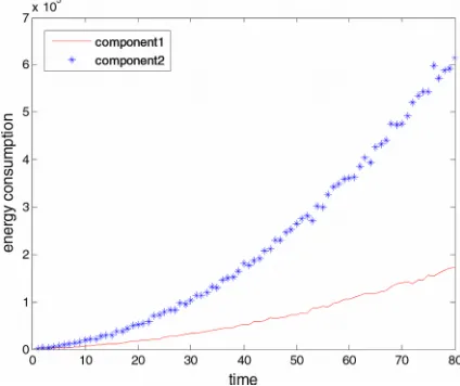
Suppose that S1 = S2 = 200, the energy consumption process of the two components are illustrated in Figure 2.
Similar to Figure 1, Figure 2 shows that the energy consumption rate of component 1 is lower than that of component 2. However, the energy consumption rate of each component is growing over time. This means that there would be much more energy consumption in the manufacture process if the components are in bad condition, even if they can still run. Therefore, we propose a new maintenance policy integrated with energy efficiency for a two-component parallel system.
The useful output during one-time unit of each component depends on its running speed as follow:
(3)
Therefore, the useful output during one-time unit of each component is constant.
Energy efficiency indicator (EEI) has been introduced in maintenance decision-making. EEI represents the amount of energy consumption needed to produce one useful output. Its mathematical expression is as follow:
(4)
Hence, energy efficiency indicator also depends on the deterioration level of components:
(5)
4. Maintenance Policy
In this section, we intend to propose a new condition-based opportunistic maintenance policy integrated with energy efficiency for a two-component parallel system. The policy is based on the following assumptions:
1. A component is not affected by the degradation of another and only the economic dependence between them is considered in this paper.
2. Inspection tasks for each component are only performed with its own fixed interval and their duration can be negligible.
3. An inspection cost of energy consumption is not higher than a deterioration inspection cost . 4. A preventive maintenance action takes place for each component when the energy efficiency indicator
exceeds its preventive maintenance threshold. The action has a specific maintenance cost for the component and a set-up cost cs.
5. If the energy efficiency indicator exceeds a legislation for component i, a corrective maintenance action is then performed. This action has a specific maintenance cost for the component and a set-up cost cs.
6. Both preventive and corrective maintenance are assumed to be perfect and the maintenance time can be ignored.
In general, both the energy consumption and deterioration level of each component can be monitored. However, Hoang et al. (2016b) point out that measuring the current deterioration level of a component is more complicated than inspecting the current energy consumption, therefore, we also assume in condition-based opportunistic maintenance policy as Hoang et al. (2016b). But we also make the additional sensitivity analysis with various and in 5.2.1 section.
In case an inspection indicates that the energy efficiency indicator of an component exceeds its legislation, the component would be considered in a rather serious state and will generate large energy consumption which would lead to a penalty, and then a corrective maintenance is performed. In order to reduce the chances of being in such serious situation, a preventive maintenance threshold lower than a legislation is considered. It should be noted that both preventive and corrective maintenance are instantaneous as Li et al. (2016). In order to comparatively analyze the minimum long-run expected cost of system per useful output unit for new proposed maintenance policy in this paper and for traditional maintenance policy as in Li et al. (2016), we also assume that the maintenance time can be negligible in this paper.
4.1. Long-Run Expected Cost of System Per Useful Output Unit
(6)
The cumulative useful output of the whole system during period (0, t] is calculated as:
(7)
Where O1 and O2 is the useful output during one time unit of component 1 and component 2 respectively.
During the period (0, t], cumulative cost of the whole system includes cumulative inspection cost, maintenance cost and energy cost:
(8)
Where:
An inspection cost of energy consumption is trigged by each inspection operation and thus ICt depends on the
number of inspection. The cumulative inspection cost of the whole system includes the inspection costs of both two components:
(9)
Similarly, MCt is related to the number of both preventive and corrective maintenance of each component. A
set-up cost and an individual maintenance cost are both generated once each maintenance (preventive or corrective) is performed. Thus, the cumulative maintenance cost of the whole system is written as:
(10)
ECt is the product of energy price and the total amount of energy consumed by the whole system:
(11)
Therefore, the cumulative cost of the whole system is the sum of Equations (9), (10) and (11), so it can finally be expressed as:
(12)
In industry, taking maintenance actions of two components jointly is more economical than repairing them separately. When a component is repaired, the cost of maintenance (both preventive and corrective) includes two parts: a fixed set-up cost cs shared by two components and individual maintenance cost of each component ( or
). Set-up cost refers to the cost resulted from the same maintenance preparation, such as maintenance devices, technology, workers and so on. Therefore, two individual preventive or corrective maintenance incur two set-up costs cs while grouping maintenance of two components only incurs single cs. Thus, a set-up cost can be saved
when two components are maintained simultaneously, which can ultimately reduce total maintenance cost and improve the economic benefit for a company. In order to make the best use of economic dependence, it is necessary to find an opportunity to postpone the preventive maintenance of one component or repair the other in advance. Hence, the cumulative cost of the whole system can be reduced by a set-up cost multiplied by the number of grouping maintenance (NGM) as follows:
4.2. A New Opportunistic Maintenance Policy Integrated with Energy Efficiency (Policy 0)
Traditional condition-based opportunistic maintenance policies do not consider energy consumption during the operation of components. In response to the enhanced awareness of energy conservation over the whole world, this paper proposes a new condition-based opportunistic maintenance decision rule by using energy efficiency indicator (EEI).
Since the actual energy consumption of components can be achieved by inspection (then EEI is calculated), we can consider the inspection time as the decision moment. Suppose that the current time is nΔT1 (the
moment of nth inspection for component 1). If the energy efficiency indicator of component 1 EEI1(nΔT1)
exceeds its preventive maintenance threshold, a maintenance action (preventive or corrective) can be performed for component 1 according to CBM decision rule. On the one hand, once the energy efficiency indicator of component 2 EEI2(nΔT1) also reaches its preventive maintenance threshold at the same time, then
we can take the preventive maintenance for component 2 in advance. On the other hand, the time of next inspection (m + 1)ΔT2 (the moment of (m + 1)th inspection for component 2) is very close to nΔT1 (see
Figure 3).
Figure 3. Sketch of inspection time
In such a situation, it is possible to postpone preventive maintenance for component 1. Although both the status of component 2 at current time and the status of component 1 at the next inspection time are unknown, we can determine the opportunistic maintenance activities by calculating two probability values in Figure 4 which details the maintenance decision process.
Pp2 = P(EEI2(nΔT1) ≥ EEIM2 | EEI2(mΔT2) = a) represents the probability that the energy efficiency indicator of
component 2 reaches its preventive threshold at current time nΔT1, under the condition that the energy efficiency
indicator of component 2 does not reach its preventive maintenance threshold at its last inspection time mΔT2 (a < EEIM2. According to Equation (5), the value of Pp2 can be obtained by firstly transforming energy
efficiency indicator of component 2 into the corresponding deterioration level, as X2(t) = f–1(t(EEI2(t)). Pp2 is
related to the last energy efficiency indicator of component 2 and it is calculated as follows:
(14)
Where X2EEI2(nΔT1) – X2a follows Gamma distribution with parameter (nΔT1 – mΔT2)α2 and β2. Then according to
Equation (1), Pp2 can be calculated as follows:
(15)
Pc1 = P(EEI1((m + 1)ΔT2) ≥ EEIL1 | EEI1(nΔT1) = b) is the probability that the energy efficiency indicator of
component 1 will exceed its legislation at the next inspection time (m + 1)ΔT2 and the current EEI of component 1
is denoted by b. Similar to Pp2, the value of Pc1 is computed as follows:
(16)
Li et al. (2016) points out that PP and PC, the threshold of Pp2 and Pc1, are difficult to compute. Therefore, PP and PC will be set in advance and they are optimized through simulation.
From Figure 4, we conclude the following six maintenance activities: • No opportunity of grouping maintenance:
1. If EEI1(nΔT1) < EEIM1, no maintenance activity will be carried out and we need to wait for the next
inspection. This means that component 1 still operates well and does not cause a great amount of energy consumption.
2. If EEIM1 ≤ EEI1(nΔT1) < EEIL1 and Pp2 ≤ PP, only a preventive maintenance of component 1 takes
place.
3. If EEI1(nΔT1) ≥ EEIL1 and Pp2 ≤ PP, only a corrective maintenance action of component 1 is
performed.
Pp2 represents the probability that component 2 needs a preventive maintenance at current time.
Obviously, taking a maintenance action of component 2 too early will increase maintenance cost (Pp2
group maintenance only when Pp2 is large enough (Pp2 > PP). If Pp2 → 1, component 2 will be
repaired immediately at the next inspection time (m + 1)ΔT2. In this case, a preventive maintenance for
component 2 is carried out in advance, in order to save one set-up cost cs and avoid the energy
efficiency indicator of component 2 beyond its legislation before next inspection time. • Opportunity of grouping maintenance is identified:
4. If EEI1(nΔT1) ≥ EEIL1 and Pp2 > PP, a corrective maintenance is performed for component 1 and
the preventive maintenance is preempted for component 2.
It’s inadvisable to postpone maintenance for component 1 when the energy efficiency indicator of component 1 exceeds its legislation. This indicates that the current energy consumption of component 1 is too large, thus component 1 must be maintained immediately. Therefore, we need to take a corrective maintenance for component 1 and preempt the preventive maintenance for component 2 at current time.
5. If EEIM1 ≤ EEI1(nΔT1) < EEIL1, Pp2 > PP and Pc1≥ PC, a preventive maintenance is performed for
component 1 and the preventive maintenance is preempted for component 2.
6. If EEIM1 ≤ EEI1(nΔT1) < EEIL1, Pp2 > PP, and Pc1 < PC, the preventive maintenance of
component 1 is postponed to the next inspection time (m + 1)ΔT2.
Pc1 is the probability that the energy efficiency indicator of component 1 will exceed its legislation at
the next inspection time (m + 1)ΔT2. An unreasonable postponed maintenance (when Pc1 is large)
maybe take a risk that the energy efficiency indicator of component 1 reaches its legislation before repaired at the next inspection time. If Pc1 → 0, then the energy efficiency indicator of component 1
will almost be lower than its legislation before the next inspection time. Therefore, the maintenance of component 1 can be postponed only when Pc1 is small enough (Pc1< PC).
Specifically, if Pp2 is small enough, it is useless to postpone maintenance for component 1, because
component 2 would hardly be repaired at the next inspection time (m + 1)ΔT2. In such case, grouping
maintenance will rarely take place at the next inspection time even if the maintenance of component 1 is postponed. Therefore, we should check the condition Pp2 > PP at first.
5. Numerical Experiments
This section will compare the proposed Policy 0 with the classical maintenance policy (Policy 1) in order to testify the superiority of Policy 0. We use Monte-Carlo method to imitate the operation process and obtain the optimum decision variables. According to Li et al. (2016), the maintenance decision rule of Policy 1 is similar to that of Policy 0. But the nature of Policy 1 is that all maintenance activities in this policy are determined by deterioration level of components, whereas Policy 0 is based on energy efficiency. Finally, the long-run expected cost of system per useful output unit of Policy 0and that of Policy 1are both estimated by Equation (6). However, it is significant to notice that the inspection cost of Policy 1 depends on deterioration inspection operation ( ), instead of energy consumption inspection cost ( ) in Equation (13). Detailed description of Policy 1 is shown in Appendix A.
5.1. Simulation Analysis
All maintenance activities in Policy 0 are determined by the energy efficiency of components. According to Equation (4), the energy efficiency indicator of component i is a function of the energy consumption and the useful output during one time unit. The energy consumption can be estimated by the non-linear fitting of some historical data from different operating status and it is expressed as (Hoang et al., 2016b):
Without loss of generality, we define Si as a constant in the range of 400 to 1200.
Meanwhile, the useful output during one time unit of component i is provided as (Hoang et al., 2016b):
(18)
Then the energy efficiency indicator of component i can be obtained based on Equations (4), (17) and (18).
In Policy 0, the decision variables are ΔT1, ΔT2, EEIM1, EEIM2, PP, PC. In Policy 1, the decision variables are ΔT1,
ΔT2, M1, M2, PP', PC'. Total time should be large enough to ensure the number of inspection and acquire more
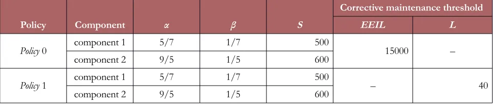
reliable results. The parameters of two policies are shown in Table 1.
Table 2 shows costs of inspection and maintenance activities, all the costs are unit cost.
For the record of computing long-run expected cost of system per useful output unit, large amount of simulation is preceded. Different combinations of decision variables can lead to different results. The optimal long-run expected cost of system per useful output unit (CO* ) and decision variables of two policies are found and
specifically shown in Table 3.
Table 3 shows that the optimal long-run expected cost of system per useful output unit of Policy 0 is 8.8046($/product). And it also presents that the optimal long-run expected cost of system per useful output unit of Policy 1 is 9.4622($/product), which is higher than that of Policy 0. Therefore, Policy 0 is superior to Policy 1 in terms of the long-run expected cost of system per useful output unit. Additional, the optimal decision variables of Policy 0 are ΔT1* = 9, ΔT2* = 8.5, PP* = 0.9, PC* = 0.05, EEIM1* = 2800(Wh/product), EEIM2* =
2750(Wh/product). The optimal decision variables of Policy 1 are ΔT1* = 10.5, ΔT2* = 9.5, PP'* = 0.88, PC'* = 0.06, M1* = 10.5, M2* = 9. Table 3 shows that PP* and PP'* are both close to 1. It also reveals that PC* and PC'* are
both close to 0. In general, the value of PP*, PP'* should be large enough and the ideal value of them are 1. But
the value of PC*, PC'* ought to be small enough and the ideal value of them are 0. Thus these results are
consistent with actual situation.
Policy Component α β S
Corrective maintenance threshold
EEIL L
Policy 0 component 1 5/7 1/7 500 15000 –
component 2 9/5 1/5 600
Policy 1 component 1 5/7 1/7 500 – 40
component 2 9/5 1/5 600
Table 1. Parameters for two policies
Policy Component cp cc cs Ep
Policy 0 component 1 80 150 100 0.025 5 –
component 2 100 200 10 –
Policy 1 component 1 80 150 100 0.025 – 10
component 2 100 200 – 15
Table 2. Data of various cost parameters
Policy CO* ΔT1* ΔT2* EEIM1* EEIM2* M1* M2* PP* PC* PP'* PC'*
Policy 0 8.8046 9 8.5 2800 2750 – – 0.9 0.05 – –
Policy 1 9.4622 10.5 9.5 – – 10.5 9 – – 0.88 0.06
5.2. Sensitivity Analysis
In order to discuss the performance of our new proposed condition-based opportunistic maintenance policy integrated with energy efficiency (Policy 0), various sensitivity analyses are carried out in the following.
5.2.1. Sensitivity Analysis to Inspection Costs
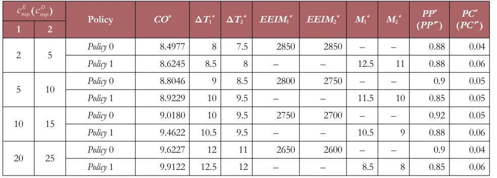
It is significant to conduct a sensitivity analysis with various and (i = 1,2). All simulation results for two policies are given in Table 4.
( )
Policy CO* ΔT1* ΔT2* EEIM1* EEIM2* M1* M2* PP*
(PP'* ) PC * (PC'* )
1 2
2 5 Policy 0 8.4977 8 7.5 2850 2850 – – 0.88 0.04
Policy 1 8.6245 8.5 8 – – 12.5 11 0.88 0.06
5 10 Policy 0 8.8046 9 8.5 2800 2750 – – 0.9 0.05
Policy 1 8.9229 10 9.5 – – 11.5 10 0.85 0.05
10 15 Policy 0 9.0180 10 9.5 2750 2700 – – 0.92 0.05
Policy 1 9.4622 10.5 9.5 – – 10.5 9 0.88 0.06
20 25 Policy 0 9.6227 12 11 2650 2600 – – 0.9 0.04
Policy 1 9.9122 12.5 12 – – 8.5 8 0.85 0.06
Table 4. CO* and optimal decision variables of two policieswith different inspection costs
5.2.2. Sensitivity Analysis to Running Speed
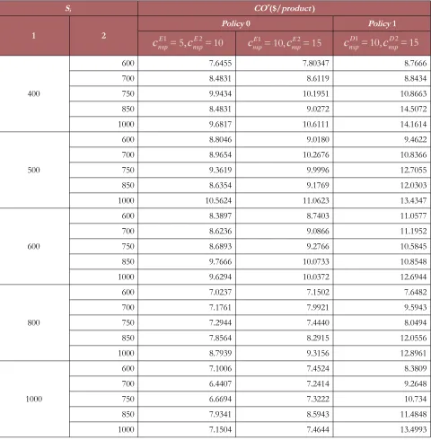
Concerning the simulation analysis and the sensitivity analysis on inspection costs above, we have concluded that Policy 0 performs better than Policy 1in terms of the long-run expected cost of system per useful output unit. Since both the energy consumption and useful output are associated with the running speed, this section makes a sensitivity analysis of the running speeds for two policies. All the optimal long-run expected costs of system per useful output unit of two policies are given in Table 5.
As shown in Table 5, when Si changes, CO* of Policy 0 fluctuates between about 6.5 and 10.5 with ,
while corresponding CO* varies between about 7.0 and 11 with . However, CO* of Policy 1 fluctuates
in the range of about 7.5 and 14.5 as Si changes. Thus it can be concluded that CO* of Policy 0 is relatively more
stable because CO* of Policy 0 varies less than that of Policy 1. Therefore, we can conclude that the maintenance
decision making by using EEI can lead to a better performance.
In addition, it is very clear that CO* of Policy 0 with is higher than that of Policy 0 with
regardless of the values of running speed.
It is significant to notice that CO* of Policy 0 is always lower than that of Policy 1 when (i = 1,2). It’s also
Si CO*($/product)
1 2
Policy 0 Policy 1
400
600 7.6455 7.80347 8.7666
700 8.4831 8.6119 8.8434
750 9.9434 10.1951 10.8663
850 8.4831 9.0272 14.5072
1000 9.6817 10.6111 14.1614
500
600 8.8046 9.0180 9.4622
700 8.9654 10.2676 10.8366
750 9.3619 9.9996 12.7055
850 8.6354 9.1769 12.0303
1000 10.5624 11.0623 13.4347
600
600 8.3897 8.7403 11.0577
700 8.6236 9.0866 11.1952
750 8.6893 9.2766 10.5845
850 9.7666 10.0733 10.8548
1000 9.6294 10.0372 12.6944
800
600 7.0237 7.1502 7.6482
700 7.1761 7.9921 9.5943
750 7.2944 7.4440 8.0494
850 7.8564 8.2915 12.0556
1000 8.7939 9.3156 12.8961
1000
600 7.1006 7.4524 8.3809
700 6.4407 7.2414 9.2648
750 6.6694 7.3222 10.734
850 7.9341 8.5943 11.4848
1000 7.1504 7.4644 13.4993
Table 5. CO* of two policies with different S1 and S 2
5.2.3. Sensitivity Analysis to Deterioration Parameter
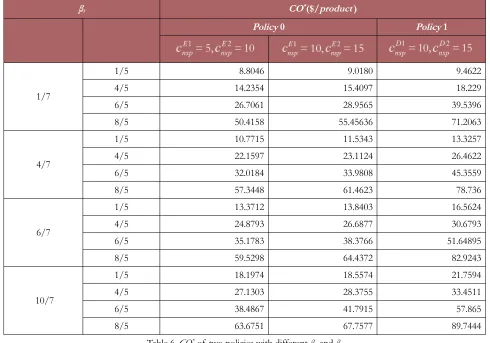
In the above sections, Policy 0 has been justified to perform better than Policy 1in terms of the long-run expected cost of system per useful output unit. This section studies the impact of variation of degradation process denoted by βi on CO* in two policies. Table 6 provides all the simulation results.
According to Table 6, as βi(i = 1,2) rise, CO* of Policy 0 increases with various (i = 1,2), as well as CO* of
Policy 1. When , , we find that Policy 0 always provides lower CO* than Policy 1 with
varying βi(i = 1,2). It is significant to notice that the superiority of Policy 0 still exists even if = 10 and
= 15.
βi CO*($/product)
Policy 0 Policy 1
1/7
1/5 8.8046 9.0180 9.4622
4/5 14.2354 15.4097 18.229
6/5 26.7061 28.9565 39.5396
8/5 50.4158 55.45636 71.2063
4/7
1/5 10.7715 11.5343 13.3257
4/5 22.1597 23.1124 26.4622
6/5 32.0184 33.9808 45.3559
8/5 57.3448 61.4623 78.736
6/7
1/5 13.3712 13.8403 16.5624
4/5 24.8793 26.6877 30.6793
6/5 35.1783 38.3766 51.64895
8/5 59.5298 64.4372 82.9243
10/7
1/5 18.1974 18.5574 21.7594
4/5 27.1303 28.3755 33.4511
6/5 38.4867 41.7915 57.865
8/5 63.6751 67.7577 89.7444
Table 6. CO* of two policies with different β1 and β 2
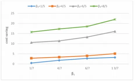
Figure 5. The cost saving with various βi when = 5, = 10
Figure 5 shows that when β2 is fixed, the cost saving increases as β1 increases. Similarly, when β1 is fixed, the larger β2
the more cost saving is. Moreover, the finding is also suitable for the cost saving when = 10 and = 15, seeing Figure 6.
Figure 6 reveals clearly that when β2 is fixed, the cost saving increases gradually as β1 rises. And it also presents that
when β1 is fixed, the cost saving also increases as β2 rises.
Above all, larger variation of degradation process (high value of βi) leads to a higher cost saving even if each energy
Figure 6. The cost savingwith various βi when = 10, = 15
6. Conclusion
In the past, some companies would not maintain the components when they could still work, even if these components were gradually in poor state which would increase energy consumption. With the enhanced awareness of energy conservation, it will be an inevitable trend to consider energy consumption in maintenance decision-making. Compared with classical maintenance policy (Policy 1), the new proposed maintenance policy (Policy 0) in this paper can save total cost including energy cost. The simulation results and sensitivity analyses show that Policy 0 always results a lower long-run expected cost of system per useful output unit than Policy 1, even if each energy consumption inspection cost equals to each deterioration inspection cost. In addition, Policy 0 always performs better than Policy 1 regardless of the value of the running speeds. Furthermore, larger variation of deterioration process leads to a higher cost saving of the whole system provided by Policy 0 compared to Policy 1. In summary, the new proposed maintenance policy in this paper performs better than the existing maintenance policy, because the new policy can save total cost including both economic and ecological costs. The new proposed policy integrated with energy efficiency in this paper helps enterprises achieve sustainable development. Therefore, in order to establish green images for companies, managers need to consider both economic cost and energy consumption when they make maintenance plans. In addition, they can integrate energy efficiency into maintenance decision-making if possible.
Although the new proposed maintenance policy performs well, there still exists some limitations. With regard to two-component parallel system, this paper only considers the economic dependence. However, stochastic dependence exists in two-component parallel systems. Furthermore, only energy consumption is considered in this paper, which is one of the ecological impacts.
On the basis of this paper, both stochastic and economic dependence will be studied in the future. Our research will also focus on applying the proposed maintenance policy into a more complex system, such as series-parallel system. Other ecological impacts, such as carbon dioxide emissions, will be studied in the future. In addition, indicators that energy efficiency and any other ecological impacts will be taken into maintenance decision-making. This would be a rather interesting research field in the future.
Declaration of Conflicting Interests
The authors declare that there is no conflict of interest regarding the publication of this paper.
Funding
The research described in this paper has been funded by the National Natural Science Foundation of China (Grant No. 71302053).
References
Barbera, F., Schneider, H., & Watson, E. (1999). A condition based maintenance model for a two-unit series system. European Journal of Operational Research, 116(2), 281-290. https://doi.org/10.1016/S0377-2217(98)00189-1
Bian, L., & Gebraeel, N. (2014). Stochastic modeling and real-time prognostics for multi-component systems with degradation rate interactions. Iie Transactions, 46(5), 470-482. https://doi.org/10.1080/0740817X.2013.812269
Bouvard, K., Artus, S., Bérenguer, C., & Cocquempot, V. (2011). Condition-based dynamic maintenance operations planning & grouping. Application to commercial heavy vehicles. Reliability Engineering & System Safety, 96(6), 601-610. https://doi.org/10.1016/j.ress.2010.11.009
Castanier, B., Grall, A., & Berenguer, C. (2005). A condition-based maintenance policy with non-periodic inspections for a two-unit series system. Reliability Engineering & System Safety, 87(1), 109-120.
https://doi.org/10.1016/j.ress.2004.04.013
Cavalcante, C.A.V., & Lopes, R.S. (2014). Opportunistic Maintenance Policy for a System with Hidden Failures: A Multicriteria Approach Applied to an Emergency Diesel Generator. Mathematical Problems in Engineering., 2014(3), 1-11. https://doi.org/10.1155/2014/157282
Chouikhi, H., Dellagi, S., & Rezg, N. (2012). Development and optimisation of a maintenance policy under environmental constraints. International Journal of Production Research, 50(13), 3612-3620.
https://doi.org/10.1080/00207543.2012.670929
Dao, C.D., & Zuo, M.J. (2017). Selective maintenance of multi-state systems with structural dependence. Reliability Engineering & System Safety, 159, 184-195. https://doi.org/10.1016/j.ress.2016.11.013
Dieulle, L., Bérenguer, C., Grall, A., & Roussignol, M. (2003). Sequential condition-based maintenance scheduling for a deteriorating system. European Journal of Operational Research, 150(2), 451-461.
https://doi.org/10.1016/S0377-2217(02)00593-3
Garg, H. (2014a). A hybrid GA-GSA algorithm for optimizing the performance of an industrial system by utilizing uncertain data in Handbook of Research on Artificial Intelligence Techniques and Algorithms (625-659). USA: IGI Global. Garg, H. (2014b). Reliability, Availability and Maintainability Analysis of Industrial Systems Using PSO and Fuzzy
Methodology. Mapan, 29(2), 115-129. https://doi.org/10.1007/s12647-013-0081-x
Garg, H. (2016). Bi-criteria optimization for finding the optimal replacement interval for maintaining the performance of the process industries in Modern Optimization Algorithms and Applications in Engineering and Economics (643-675). USA.
Garg, H., Rani, M., & Sharma, S.P. (2013). Preventive maintenance scheduling of the pulping unit in a paper plant. Japan Journal of Industrial & Applied Mathematics, 30(2), 397-414. https://doi.org/10.1007/s13160-012-0099-4
Garg, H., Rani, M., Sharma, S.P., & Vishwakarma, Y. (2014a). Bi-objective optimization of the reliability-redundancy allocation problem for series-parallel system. Journal of Manufacturing Systems, 33(2), 353-367.
https://doi.org/10.1016/j.jmsy.2014.02.008
Garg, H., Rani, M., Sharma, S.P., & Vishwakarma, Y. (2014b). Intuitionistic fuzzy optimization technique for solving multi-objective reliability optimization problems in interval environment. Expert Systems with Applications, 41(7), 3157-3167. https://doi.org/10.1016/j.eswa.2013.11.014
Garg, H., & Sharma, S.P. (2012). A two-phase approach for reliability and maintainability analysis of an industrial system. International Journal of Reliability Quality & Safety Engineering, 19(03), 155-445.
https://doi.org/10.1142/S0218539312500131
Garg, H., & Sharma, S.P. (2013). Multi-objective reliability-redundancy allocation problem using particle swarm optimization. Computers & Industrial Engineering, 64(1), 247-255. https://doi.org/10.1016/j.cie.2012.09.015
Hoang, A., Do, P., & Iung, B. (2016b). Investigation on the use of energy efficiency for condition-based maintenance decision-making. IFAC-PapersOnLine, 49(28), 73-78. https://doi.org/10.1016/j.ifacol.2016.11.013
Hoang, A., Do, P., & Iung, B. (2017). Energy efficiency performance-based prognostics for aided maintenance decision-making: Application to a manufacturing platform. Journal of Cleaner Production, 142, 2838-2857.
https://doi.org/10.1016/j.jclepro.2016.10.185
Horenbeek, A.V., Kellens, K., Pintelon, L., & Duflou, J.R. (2014). Economic and Environmental Aware Maintenance Optimization. Procedia Cirp, 15, 343-348. https://doi.org/10.1016/j.procir.2014.06.048
Jardine, A.K.S., Lin, D., & Banjevic, D. (2006). A review on machinery diagnostics and prognostics implementing condition-based maintenance. Mechanical Systems & Signal Processing, 20(7), 1483-1510.
https://doi.org/10.1016/j.ymssp.2005.09.012
Jiang, X., Duan, F., Tian, H., & Wei, X. (2015). Optimization of reliability centered predictive maintenance scheme for inertial navigation system. Reliability Engineering & System Safety, 140, 208-217.
https://doi.org/10.1016/j.ress.2015.04.003
Keizer, M.C.A.O., Teunter, R.H., & Veldman, J. (2016). Clustering condition-based maintenance for systems with redundancy and economic dependencies. European Journal of Operational Research, 251(2), 531-540.
https://doi.org/10.1016/j.ejor.2015.11.008
Li, H., Deloux, E., & Dieulle, L. (2016). A condition-based maintenance policy for multi-component systems with Lévy copulas dependence. Reliability Engineering & System Safety, 149, 44-55.
https://doi.org/10.1016/j.ress.2015.12.011
Mora, M., Vera, J., Rocamora, C., & Abadia, R. (2013). Energy Efficiency and Maintenance Costs of Pumping Systems for Groundwater Extraction. Water Resources Management, 27(12), 4395-4408.
https://doi.org/10.1007/s11269-013-0423-z
Nguyen, K.A., Do, P., & Grall, A. (2014). Condition-based maintenance for multi-component systems using importance measure and predictive information. International Journal of Systems Science Operations & Logistics, 1(4), 228-245. https://doi.org/10.1080/23302674.2014.983582
Noortwijk, J.M.V. (2009). A survey of the application of gamma processes in maintenance. Reliability Engineering & System Safety, 94(1), 2-21. https://doi.org/10.1016/j.ress.2007.03.019
Qian, X., & Wu, Y. (2014). Dynamic Control-limit Policy of Condition based Maintenance for the Hydroelectricity Generating Unit. International Journal of Security & Its Applications, 8(2), 95-106.
https://doi.org/10.14257/ijsia.2014.8.2.10
Shi, H., & Zeng, J. (2016). Real-time prediction of remaining useful life and preventive opportunistic maintenance strategy for multi-component systems considering stochastic dependence. Computers & Industrial Engineering, 93, 192-204. https://doi.org/10.1016/j.cie.2015.12.016
Tian, Z., Jin, T., Wu, B., & Ding, F. (2011). Condition based maintenance optimization for wind power generation systems under continuous monitoring. Renewable Energy, 36(5), 1502-1509.
https://doi.org/10.1016/j.renene.2010.10.028
Tian, Z., & Liao, H. (2011). Condition based maintenance optimization for multi-component systems using proportional hazards model. Reliability Engineering & System Safety, 96(5), 581-589.
https://doi.org/10.1016/j.ress.2010.12.023
Tlili, L., Radhoui, M., & Chelbi, A. (2015). Condition-Based Maintenance Strategy for Production Systems Generating Environmental Damage. Mathematical Problems in Engineering, 2015, 1-12.
https://doi.org/10.1155/2015/494162
Wijnmalen, D.J.D., & Hontelez, J.A.M. (1997). Coordinated condition-based repair strategies for components of a multi-component maintenance system with discounts. European Journal of Operational Research, 98(1), 52-63.
Xu, W., & Cao, L. (2014). Energy efficiency analysis of machine tools with periodic maintenance. International Journal of Production Research, 52(18), 5273-5285. https://doi.org/10.1080/00207543.2014.893067
Zhang, Z., Zhou, Y., Sun, Y., & Ma, L. (2012). Condition-based maintenance optimisation without a predetermined strategy structure for a two-component series system. Eksploatacja i Niezawodnosc - Maintenance and Reliability, 14(2), 120-129.
Zhu, Q., Peng, H., & Houtum, G.J.V. (2015). A condition-based maintenance policy for multi-component systems with a high maintenance setup cost. Or Spectrum, 37(4), 1007-1035. https://doi.org/10.1007/s00291-015-0405-z
Appendix A
Policy 1
An existed classic condition-based opportunistic maintenance policy is extended by considering the energy consumption during the operation of the whole system. We named the extended classic maintenance policy as Policy 1. The maintenance decision rule of Policy 1 is similar to that of Policy 0. But the nature of Policy 1 is that all maintenance activities in this policy are determined by deterioration level of components.
Suppose that the current time is nΔT1 as in Figure 3 above (the moment of nth inspection for component 1). Six
kinds of maintenance activity in Policy 1 are concluded in the following: • No opportunity of grouping maintenance:
1. If X1(nΔT1) < M1 no maintenance activity will be carried out and we need to wait for the next
inspection. This means that component 1 still operates well.
2. If M1 ≤ X1(nΔT1) < L1 and Pp2 ≤ PP', only a preventive maintenance of component 1 takes place.
3. If X1(nΔT1) ≥ L1 and Pp2 ≤ PP', only a corrective maintenance action of component 1 is performed.
In this situation, we can consider that the component 1 fails.
Pp2 represents the probability that a preventive maintenance of component 2 takes place at current
time. In this policy, it refers the probability that degradation level of component 2 reaches its preventive maintenance threshold at current time. Obviously, taking a maintenance action of component 2 too early will increase maintenance cost (Pp2 is too small). Therefore, no maintenance
action will take place when Pp2 ≤ PP'. It’s worthy to take group maintenance only when Pp2 is large
enough (Pp2 > PP' ).
• Opportunity of grouping maintenance is identified:
4. If X1(nΔT1) < L1 and Pp2 > PP', a corrective maintenance is performed for component 1 and the
preventive maintenance is preempted for component 2.
5. If M1 ≤ X1(nΔT1) < L1, Pp2 > PP', and Pc1 ≥ PC', a preventive maintenance is performed for
component 1 and the preventive maintenance is preempted for component 2.
6. If M1 ≤ X1(nΔT1) < L1, Pp2 > PP', and Pc1 < PC', the preventive maintenance of component 1 is
postponed to the next inspection time (m + 1)ΔT2.
In this policy, Pc1 is the probability that component 1 will fail at the next inspection time (m + 1)ΔT2.
An unreasonable postponed maintenance (when Pc1 is large) maybe take a risk that component may
fail before repaired at the next inspection time. If Pc1 → 1, then component 1 will hardly fail before
the next inspection time. Therefore, the maintenance of component 1 can be postponed only when Pc1 is small enough (Pc1<PC').
In this policy, the long-run expected cost of system per useful output unit is also Equation (6) above:
Where:
The cumulative useful output of the whole system is Equation (7) above:
(7)
Cumulative cost of the whole system includes cumulative inspection cost, maintenance cost and energy cost. It depends on the number of deterioration inspection, preventive maintenance and corrective maintenance, as well as total amount of energy consumption. Its mathematic expression is as the following:
(19)
It should be noted that the inspection cost of Policy 1 depends on deterioration inspection operation ( in Equation(19)), instead of energy consumption inspection cost( ) in Equation (13).
Journal of Industrial Engineering and Management, 2018 (www.jiem.org)
Article’s contents are provided on an Attribution-Non Commercial 4.0 Creative commons International License. Readers are allowed to copy, distribute and communicate article’s contents, provided the author’s and Journal of Industrial Engineering and