Dynamic Conditional Correlation Analysis of Stock Market Contagion: Evidence from the 2007-2010 Financial Crises

(1)

ISSN: 2146-4138 www.econjournals.com

637

Dynamic Conditional Correlation Analysis of Stock Market Contagion:

Evidence from the 2007-2010 Financial Crises

Zouheir Mighri

Department of Quantitative Methods and Information Technology, Institut Supérieur de Gestion de Sousse, University of Sousse, Tunisia.

Laboratoire de Recherche en Economie, Management et Finance Quantitative (LREMFQ) Route Hzamia Sahloul 3 - B.P. 40 - 4054 Sousse, Tunisia.

Tel: +216 24 93 29 18. E-mail: zmighri@gmail.com

Faysal Mansouri

Department of Economics and Quantitative Methods.

Institut des Hautes Etudes Commerciales de Sousse, University of Sousse, Tunisia. Laboratoire de Recherche en Economie, Management et Finance Quantitative (LREMFQ)

Route Hzamia Sahloul 3 - B.P. 40 - 4054 Sousse, Tunisia. Tel: +216 20 33 73 06. E-mail: faysal.mansouri@fsegt.rnu.tn

ABSTRACT: This research examines the time-varying conditional correlations to the daily stock index returns. We use a dynamic conditional correlation (DCC) multivariate GARCH model in order to capture potential contagion effects between US and major developed and emerging stock markets during the 2007-2010 major financial crisis. Empirical results show substantial evidence of significant increase in conditional correlation or contagion as well as herding behavior during crisis periods. This result contrasts with the “no contagion” finding reached by Forbes and Rigobon (2002).

Keywords: Dynamic correlation; DCC-GARCH; contagion; financial crisis; stock markets.

JEL Classifications: C58

1. Introduction

The financial contagion1 phenomenon has become more pronounced especially with the 2007 subprime crisis and 2008 stock market crash. Indeed, the subprime mortgage crisis is an ongoing real estate and financial crisis triggered by a dramatic rise in mortgage delinquencies and foreclosures in the United States, with major adverse consequences for banks and financial markets around the globe. The crisis became apparent in 2007 and has exposed pervasive weaknesses in financial industry regulation and global financial system.

Definition of financial contagion phenomenon is one of the most debated themes in the literature. In this paper, we use the definition advanced by Forbes and Rigobon (2002): contagion is a significant increase in the cross-market correlation during a turmoil period. Therefore, it seems important to compare the correlation between two stock markets during relatively pre-crisis period to the during a crisis period. If two markets are moderately correlated during the pre-crisis or stable period and a shock to one stock market leads to a significant increase in market co-movement, this would generate financial contagion. Nevertheless, if two stock markets are highly correlated during the stable period, even if they continue to be highly correlated after a shock to one market, this may not generate financial contagion. Otherwise, if the correlation does not increase significantly, this co-movement between stock markets refers to strong real linkages between markets and is called interdependence (Forbes and Rigobon, 2002).

1

(2)

638 The financial contagion with its serious consequences has become an integral part and concern of the activity in international equity markets. The 2007 subprime crisis have led to fragile international stock markets. In this article, we attempt to understand and model the volatility of these markets that are constantly growing in order to anticipate and contain the huge negative consequences of this crisis. The portfolio managers of financial assets rely on correlations estimators between the returns of these assets and the volatility of those returns. The task seems relatively easy in the case where correlations and volatilities are not time-varying. However, reality suggests dynamic correlations and volatilities do vary with time, in particular during crises periods.

In this paper, we extend the adjusted correlation analysis of Forbes and Rigobon (2002) by considering the dynamic conditional correlation model (DCC-GARCH) of Engle (2002) that significantly improves the Constant Conditional Correlation (CCC-GARCH) model of Bollerslev (1990).With the DCC model, the constant correlation assumption is relaxed by allowing for the time-varying correlation, and the number of unknown parameters is limited (see also Engle and Sheppard (2001) and Tse and Tsui (1999, 2002), among others). The recognition of time dependence characteristic through the multivariate modeling structure may lead to more interesting empirical results than working with separate univariate models (see Bauwens and Laurent (2005) and Bauwens et al. (2006), among others).The multivariate DCC-GARCH approach increasingly being used as the most popular model of time-varying correlations amongst other multivariate GARCH models. Kearney and Patton (2000) and Karolyi (1995) argue that the most obvious application of these models is the study of relationships between the volatilities and co-volatilities of several financial markets.

The application of DCC-type models has recently become a key focus of financial econometrics as the threads of the widespread contagion of financial crises which are likely to occur at any time due to the potential collapse of diverse stock market indices. In the literature, some papers test the existence of contagion effects on stock markets (see Chiang et al. (2007) and Syllignakis and Kouretas (2011), among others) by using the DCC-GARCH type models. Several questions arise naturally:

 Does the correlation between financial asset returns vary over time?

 Does this correlation increase during financial crises periods?

 Is there a contagion phenomenon during the 2007-2010 financial crisis?

These issues may be tackled through multivariate models and increase the query on the specification of the covariances or correlations dynamics. In this paper, we model the volatility in a multivariate structure that incorporates dynamic correlations. The main objective is to model financial contagion phenomenon using the multivariate DCC-GARCH model of Engle (2002). The major advantage of employing this approach is the detection of potential changes in time-varying conditional correlations, which allows us to capture dynamic investor behavior in response to news and innovations. Furthermore, the dynamic conditional correlations measure is suitable to examine possible contagion effects due to herding behavior in emerging stock markets during turmoil periods [see Corsetti et al. (2005), Boyer et al. (2006), Chiang et al. (2007), Syllignakis and Kouretas (2011) and Celik (2012)].

The remainder of the paper is organized as follows. Section 2 discusses the database and the descriptive statistics. Section 3 focuses on identifying the financial contagion phenomenon by using the simple and adjusted correlation analysis of Forbes and Rigobon (2002). Section 4 introduces the econometric methodology of the multivariate DCC-GARCH model and provides the main empirical results. Section 5 summarizes the findings and indicates further research directions.

2. Database and Descriptive Statistics

In this paper, we use daily stock price indices data base2. The sample period for all data is from January 1, 2003 to December 31, 2010. The stock market indices used are S&P500 for the USA, CAC40 for France, DAX for Germany, FTSE100 for the United-Kingdom, AEX for Netherlands, ATX for Austria, IBOVESPA for Brazil, BSE30 for India, HSI for Hong Kong, IPC for Mexico, JKSE for Indonesia, KLSE for Malaysia, MERVAL for Argentina, OMXC20 for Denmark, SCI

2

(3)

639 (CHINA SHANGHAI COMPOSITE INDEX) for China, SSMI for Switzerland and STI for Singapore. The daily stock index returns are defined as logarithmic differences of stock price indices and thus computed as = 100 ln( / ) for = 1,2, … , where , , and are the total number of observations, the return at time , the current stock price index and the lagged day’s stock price index, respectively. The reason for multiplying the expression ln ( / ) by 100 is due to numerical problems in the estimation part. This will not affect the structure of the model since it is just a linear scaling.

Tables 1 and 2 report summary statistics for the stock return series during the entire period, before and after the 2007 subprime crisis. During the full sample period, the MERVAL index is the most volatile, as measured by the standard deviation of 1.6013%, while the KLSE index is the least volatile with a standard deviation of 1.0081%. The measure for skewness shows that stock returns are negatively skewed with the exception of CAC40, DAX, HSI, IPC and SSMI returns that are positively skewed. The negative skewness indicates that large negative stock returns are more common than large positive returns. From the measure for Excess Kurtosis, the leptokurtic behavior is apparent in all series with more pronounced fat tails in S&P500 and KLSE returns. This implies that large shocks of either sign are more likely to be present and that the stock-return series may not be normally distributed.

Also, the Jarque-Bera statistics indicate that the assumption of normality is rejected decisively for all stock return series. The non-normality is apparent from the fatter tails from the normal distribution and mild negative and positive skewness. Moreover, the Box-Pierce test of serial correlation on the standardized residuals show that all stock return series exhibit significant autocorrelation. Besides, the significance of the Box-Pierce test statistics on the squared standardized residuals tells us that ARCH effects are still there. The existence of such serial correlation may be explained by the non-synchronous trading of the stocks or to some form of market inefficiency, producing a partial adjustment process. The statistical significance of the ARCH-Fisher test statistics confirms the existence of autoregressive conditional heteroskedasticity (ARCH) in the stock return and squared return series.

Table1.Descriptive statistics on stock returns

S&P500 AEX ATX IBOVESPA CAC40 DAX FTSE100 HSI IPC

Panel A: The entire period: 01/01/2003 to 31/12/2010 (2922 observations)

Mean 0,0122 0,0032 0,0317 0,0622 0,0074 0,0298 0,0138 0,031 0,0629

Std.dev 1,1149 1,2828 1,3781 1,5886 1,2297 1,2356 1,0615 1,372 1,1619

Minimum -9,4695 -9,5903 -10,253 -12,096 -9,4715 -7,4335 -9,2646 -13,582 -7,2661

Maximum 10,957 10,028 12,021 13,678 10,595 10,797 9,3842 13,407 10,441

Skewness -0,2903* -0.0425* -0.3589* -0,0454 0,1681* 0,1764* -0,0894** 0,1114** 0,1712* (0,0000) (0,0000) (0,0000) (0,3158) (0,0002) (0,0001) (0,0485) (0,0139) (0,0002) Excess Kurtosis 17,079* 12.638* 11.831* 8,9622* 12,209* 10,911* 13,820* 15,586* 9,5176*

(0,0000) (0,0000) (0,0000) (0,0000) (0,0000) (0,0000) (0,0000) (0,0000) (0,0000)

Jarque-Bera 35556* 19447* 17105* 9780* 18162* 14510* 23257* 29581* 11043*

(0,0000) (0,0000) (0,0000) (0,0000) (0,0000) (0,0000) (0,0000) (0,0000) (0,0000) ARCH(10) 84,602* 90.569* 64.704* 70,245* 61,515* 47,197* 73,232* 68,354* 48,120*

(0,0000) (0,0000) (0,0000) (0,0000) (0,0000) (0,0000) (0,0000) (0,0000) (0,0000) (50) 214,726* 124.608* 173.501* 105,276* 134,452* 112,409* 169,356* 162,516* 90,616*

(0,0000) (0,0000) (0,0000) (0,0000) (0,0000) (0,0000) (0,0000) (0,0000) (0,0004) (50) 5107,060* 3699.98* 5084.40* 3733,890* 2567,920* 2351,650* 3559,010* 3132,800* 2560,120*

(0,0000) (0,0000) (0,0000) (0,0000) (0,0000) (0,0000) (0,0000) (0,0000) (0,0000)

Panel B: Before the crisis: 01/01/2003 to 31/07/2007 (1673 observations)

Mean 0,0301 0,0301 0,084 0,0939 0,0376 0,0576 0,0286 0,0545 0,0962

Std.dev 0,6496 0,9906 0,8237 1,319 0,886 1,0294 0,6991 0,7958 0,9271

Minimum -3,5867 -6,5956 -7,7676 -6,8566 -5,8345 -6,336 -4,9181 -4,1836 -5,9775

Maximum 3,4814 9,5169 4,6719 5,1615 7,0023 7,086 5,9038 3,5998 6,5101

Skewness -0,0219 0,2979* -1,0182* -0,253* 0,0295 0,0245 0,0186 -0,1649* -0,1263** (0,7149) (0,0000) (0,0000) (0,0000) (0,6225) (0,6822) (0,7560) (0,0059) (0,0348) Excess Kurtosis 3,8571* 12,300* 10,138* 2,4881* 7,4961* 6,744* 7,7969* 3,3575* 5,3126*

(0,0000) (0,0000) (0,0000) (0,0000) (0,0000) (0,0000) (0,0000) (0,0000) (0,0000) Jarque-Bera 1037,200* 10571* 7453,500* 449,400* 3917,200* 3170,600* 4237,800* 793,390* 1971,900*

(0,0000) (0,0000) (0,0000) (0,0000) (0,0000) (0,0000) (0,0000) (0,0000) (0,0000) ARCH(10) 23,155* 45,639* 13,553* 8,277* 39,140* 26,356* 41,186* 4,802* 14,152*

(4)

640

(50) 62,8698 158,922* 77,9634* 50,1527 101,480* 110,810* 110,029* 48,3018 71,959** (0,1045) (0,0000) (0,0069) (0,4673) (0,0000) (0,0000) (0,0000) (0,5418) (0,0226) (50) 709,170* 2126,430* 430,203* 392,778* 1328,320* 1767,600* 1273,370* 316,084* 697,154*

(0,0000) (0,0000) (0,0000) (0,0000) (0,0000) (0,0000) (0,0000) (0,0000) (0,0000)

Panel C: After the crisis:01/08/2007 to 31/12/2010 (1249 observations)

Mean -0,0117 -0,0328 -0,0383 0,0197 -0,0331 -0,0074 -0,006 -0,0005 0,0183

Std.dev 1,5303 1,5916 1,8777 1,8895 1,5759 1,4662 1,4074 1,8852 1,4154

Minimum -9,4695 -9,5903 -10,253 -12,096 -9,4715 -7,4335 -9,2646 -13,582 -7,2661

Maximum 10,957 10,028 12,021 13,678 10,595 10,797 9,3842 13,407 10,441

Skewness -0,222* -0,1067 -0,1265 0,0867 0,2326* 0,2743* -0,0609 0,1583** 0,3231* (0,0013) (0,1234) (0,0677) (0,2107) (0,0008) (0,0001) (0,3788) (0,0222) (0,0000) Excess Kurtosis 9,9216* 9,3434* 6,4004* 9,2467* 8,8067* 10,264* 8,8491* 8,9374* 8,2841*

(0,0000) (0,0000) (0,0000) (0,0000) (0,0000) (0,0000) (0,0000) (0,0000) (0,0000) Jarque-Bera 5133,200* 4545,500* 2135,200* 4451,200* 4047,500* 5497,800* 4075,900* 4162,200* 3593,200*

(0,0000) (0,0000) (0,0000) (0,0000) (0,0000) (0,0000) (0,0000) (0,0000) (0,0000) ARCH(10) 31,898* 43,140* 23,279* 34,247* 25,542* 19,478* 29,412* 25,861* 21,157*

(0,0000) (0,0000) (0,0000) (0,0000) (0,0000) (0,0000) (0,0000) (0,0000) (0,0000) (50) 133,998* 107,351* 110,049* 91,563* 109,365* 111,703* 112,246* 105,164* 72,683**

(0,0000) (0,0000) (0,0000) (0,0003) (0,0000) (0,0000) (0,0000) (0,0000) (0,0197) (50) 1723,750* 1421,570* 1665,950* 1721,070* 861,560* 862,784* 1206,910* 969,661* 1052,800*

(0,0000) (0,0000) (0,0000) (0,0000) (0,0000) (0,0000) (0,0000) (0,0000) (0,0000)

Notes: Observations for all series in the whole sample period are 2922. The observations for the pre-crisis (01/01/200307/31/2007) and post-crisis (08/01/200712/31/2010) sub-periods are 1673 and 1249, respectively. * and ** denote statistical significance at the 1% and 5% levels, respectively. All variables are first differences of the natural log of stock indices times 100. ( )and ( )refer to Ljung-Box statistics for returns and squared returns, respectively, with up to 50-day lags.

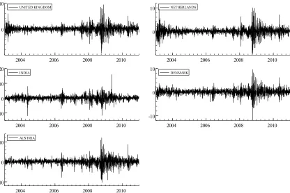
To provide more insights into stock market interactive linkages during the period under study, we depict in Figure 1 their stock returns over time. The first impression is that the stock returns almost follow a similar movement. With the exception of Malaysia, the plots show a clustering of larger return volatility around and after 2007. This means that the indices are characterized by volatility clustering, i.e., large (small) volatility tends to be followed by large (small) volatility, revealing the presence of heteroskedasticity. This market phenomenon has been widely recognized and successfully captured by ARCH/GARCH family models to adequately describe stock market returns volatility dynamics. This is important because the econometric model will be based on the interdependence of the stock markets in the form of second moments by modeling the time varying variance-covariance matrix for the sample.

Table2.Descriptive statistics on stock returns (continued).

JKSE KLSE MERVAL OMXC20 SCI BSE30 SSMI STI

Panel A: The entire period: 01/01/2003 to 31/12/2010 (2922 observations)

Mean 0,0741 0,0292 0,0652 0,0284 0,0249 0,0617 0,0113 0,0297

Std.dev 1,2552 1,0081 1,6013 1,1392 1,4682 1,4341 1,0153 1,0612

Minimum -10,954 -19,246 -12,952 -11,723 -9,2562 -11,809 -8,1078 -9,2155

Maximum 7,6234 19,860 10,432 9,4964 9,0343 15,990 10,788 7,5305

Skewness -0,6292* -0,1284* -0,6554* -0,2719* -0,307* -0,0733 0,1002** -0,3787* (0,0000) (0,0046) (0,0000) (0,0000) (0,0000) (0,1058) (0,0270) (0,0000) Excess Kurtosis 10,365* 158,650* 8,1629* 11,972* 6,0603* 12,398* 12,457* 10,567*

(0,0000) (0,0000) (0,0000) (0,0000) (0,0000) (0,0000) (0,0000) (0,0000) Jarque-Bera 13274* 3064500* 8321,700* 17485* 4517,5* 18716* 18897* 13664*

(0,0000) (0,0000) (0,0000) (0,0000) (0,0000) (0,0000) (0,0000) (0,0000) ARCH(10) 32,287* 179,100* 58,886* 97,944* 13,727* 20,314* 104,410* 45,890*

(0,0000) (0,0000) (0,0000) (0,0000) (0,0000) (0,0000) (0,0000) (0,0000) (50) 91,159* 404,704* 77,455* 119,259* 114,397* 121,902* 154,006* 137,277*

(0,0003) (0,0000) (0,0077) (0,0000) (0,0000) (0,0000) (0,0000) (0,0000) (50) 979,404* 1357,020* 1927,870* 3404,790* 782,756* 860,764* 3393,510* 2431,220*

(0,0000) (0,0000) (0,0000) (0,0000) (0,0000) (0,0000) (0,0000) (0,0000)

Panel B: Before the crisis: 01/01/2003 to 31/07/2007 (1673 observations)

Mean 0,1022 0,0451 0,0851 0,0549 0,0712 0,0913 0,0390 0,0582

Std.dev 1,0187 0,5644 1,4118 0,7753 1,2094 1,1523 0,7808 0,7496

Minimum -7,8002 -4,7465 -9,0215 -4,1651 -9,2562 -11,8090 -5,1278 -4,0367

(5)

641

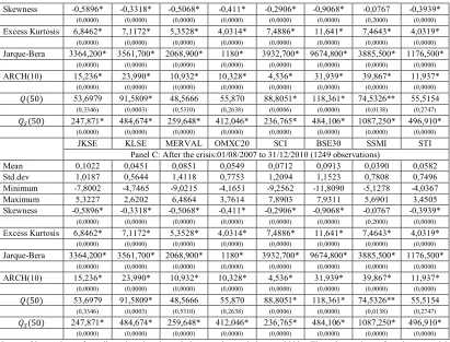
Skewness -0,5896* -0,3318* -0,5068* -0,411* -0,2906* -0,9068* -0,0767 -0,3939* (0,0000) (0,0000) (0,0000) (0,0000) (0,0000) (0,0000) (0,2000) (0,0000) Excess Kurtosis 6,8462* 7,1172* 5,3528* 4,0314* 7,4886* 11,641* 7,4643* 4,0319*

(0,0000) (0,0000) (0,0000) (0,0000) (0,0000) (0,0000) (0,0000) (0,0000) Jarque-Bera 3364,200* 3561,700* 2068,900* 1180* 3932,700* 9674,800* 3885,500* 1176,500*

(0,0000) (0,0000) (0,0000) (0,0000) (0,0000) (0,0000) (0,0000) (0,0000) ARCH(10) 15,236* 23,990* 10,932* 10,328* 4,536* 31,939* 39,867* 11,937*

(0,0000) (0,0000) (0,0000) (0,0000) (0,0000) (0,0000) (0,0000) (0,0000) (50) 53,6979 91,5809* 48,5666 55,870 88,8051* 118,361* 74,5326** 55,5154

(0,3346) (0,0003) (0,5310) (0,2638) (0,0006) (0,0000) (0,0138) (0,2747) (50) 247,871* 484,674* 259,648* 412,046* 236,765* 484,106* 1087,250* 496,910*

(0,0000) (0,0000) (0,0000) (0,0000) (0,0000) (0,0000) (0,0000) (0,0000)

Panel C: After the crisis:01/08/2007 to 31/12/2010 (1249 observations)

Mean 0,1022 0,0451 0,0851 0,0549 0,0712 0,0913 0,0390 0,0582

Std.dev 1,0187 0,5644 1,4118 0,7753 1,2094 1,1523 0,7808 0,7496

Minimum -7,8002 -4,7465 -9,0215 -4,1651 -9,2562 -11,8090 -5,1278 -4,0367

Maximum 5,3227 2,6202 6,4864 3,7614 7,8903 7,9311 5,6901 3,4505

Skewness -0,5896* -0,3318* -0,5068* -0,411* -0,2906* -0,9068* -0,0767 -0,3939* (0,0000) (0,0000) (0,0000) (0,0000) (0,0000) (0,0000) (0,2000) (0,0000) Excess Kurtosis 6,8462* 7,1172* 5,3528* 4,0314* 7,4886* 11,641* 7,4643* 4,0319*

(0,0000) (0,0000) (0,0000) (0,0000) (0,0000) (0,0000) (0,0000) (0,0000) Jarque-Bera 3364,200* 3561,700* 2068,900* 1180* 3932,700* 9674,800* 3885,500* 1176,500*

(0,0000) (0,0000) (0,0000) (0,0000) (0,0000) (0,0000) (0,0000) (0,0000) ARCH(10) 15,236* 23,990* 10,932* 10,328* 4,536* 31,939* 39,867* 11,937*

(0,0000) (0,0000) (0,0000) (0,0000) (0,0000) (0,0000) (0,0000) (0,0000) (50) 53,6979 91,5809* 48,5666 55,870 88,8051* 118,361* 74,5326** 55,5154

(0,3346) (0,0003) (0,5310) (0,2638) (0,0006) (0,0000) (0,0138) (0,2747) (50) 247,871* 484,674* 259,648* 412,046* 236,765* 484,106* 1087,250* 496,910*

(0,0000) (0,0000) (0,0000) (0,0000) (0,0000) (0,0000) (0,0000) (0,0000)

Notes: Observations for all series in the whole sample period are 2922. The observations for the pre-crisis (01/01/200307/31/2007) and post-crisis (08/01/200712/31/2010) sub-periods are 1673 and 1249, respectively. * and ** denote statistical significance at the 1% and 5% levels, respectively. All variables are first differences of the natural log of stock indices times 100. ( )and ( )refer to Ljung-Box statistics for returns and squared returns, respectively, with up to 50-day lags.

As observed by various economists and financiers, the international financial crisis from 2007 to the present is considered to be the worst financial crisis since the great depression of the 1930s. The subprime crisis erupted in the second half of 2006 with the collapse of subprime in the United States where the borrowers were not able to repay. In July 2007, it turned into open crisis. The financial crisis started in 2007 and continues till 2011 marked by a liquidity crisis or a solvency crisis and a credit crunch. The crisis has triggered in July 2007 following the bursting of asset price bubbles (including the U.S. housing bubble of the 2000s) and substantial losses of financial institutions caused by the subprime crisis.

September 2008 has been marked by a fall in equity markets and the collapse of several financial institutions, causing an early systemic crisis and a deep global economic recession. The 2008 financial crisis may be considered as a second phase in the 2007-2010 financial crisis following the major 2007 subprime crisis. This second phase started during early September 2008 and affects directly or indirectly most of the countries. It promptly passed on to international stock markets increasing uncertainties, falling prices and rising the likelihood of financial crash in autumn 2008. We use August 01, 2007 as the date that splits our sample into two sub-periods: pre-crisis and post-crisis. Comparing the before and after crisis periods, we notice that stock returns are higher before the 2007 subprime crisis, while volatilities are higher after the crisis.

(6)

642

Table 3. Unconditional correlation matrix for the stock returns.

S&P500 AEX ATX IBOVESPA CAC40 DAX FTSE100 HSI IPC JKSE KLSE MERVAL OMXC20 SCI BSE30 SSMI STI

(7)

643

2004 2006 2008 2010

0

10 USA

2004 2006 2008 2010

0

10 FRANCE

2004 2006 2008 2010

0

10 GERMANY

2004 2006 2008 2010

-10 0 10

HONG KONG

2004 2006 2008 2010

-5 0 5 10

SINGAPORE

2004 2006 2008 2010

0

10 MEXICO

2004 2006 2008 2010

-10 0

10 ARGENTINA

2004 2006 2008 2010

-10 0 10

BRAZIL

2004 2006 2008 2010

0

10 SWITZERLAND

2004 2006 2008 2010

-5 0 5 10

CHINA

2004 2006 2008 2010

0 20

MALAYSIA

2004 2006 2008 2010

-10 0

(8)

644

Figure 1.Plots of daily stock market returns. 3. Simple and Adjusted Correlation Analysis

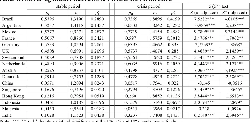
In order to measure the financial contagion phenomenon, we recourse to the simple Pearson correlation approach (see King and Wadhwani (1990), Bertero and Mayer (1990), Lee and Kim (1993), Calvo and Reinhart (1996), Baig and Goldfajn (1999) and Loretan and English (2000), among others).If the correlations significantly increase during a particular crisis period compared to a pre-crisis one (stability period), one may conclude the existence of a strengthening of links or transmission mechanisms of shocks between two markets (or group of markets) and thus detecting elements of contagion in financial markets. If the increase is not statistically significant, this indicates only an interdependence phenomenon rather than financial contagion.

Forbes and Rigobon (2002) argue that analysts need to be careful in the interpretation of the increases in simple correlations as evidence of financial contagion. This is attributable to the fact that returns correlations could increase when stock markets become highly volatile. The authors have proposed a correction of the correlation coefficients for the heteroskedasticity effect by a statistical adjustment for the conditional heteroskedasticity. Forbes and Rigobon (2002) propose to adjust the correlation coefficients in the following way:

∗₌

( ) (1)

where

 = : the unadjusted correlation coefficient between a crisis market and non-crisis market

;

 ∗: the adjusted correlation coefficient;

 = − 1: change in high period (crisis period) volatility against the low period (stability

period) volatility;

To compute the adjusted correlation coefficients, the crisis (turmoil) period is used as the high volatility period and the stable period as the low volatility period. The following hypothesis is then tested:

2004 2006 2008 2010

0 10

UNITED KINGDOM

2004 2006 2008 2010

0

10 NETHERLANDS

2004 2006 2008 2010

-10 0 10 20

INDIA

2004 2006 2008 2010

-10 0 10

DENMARK

2004 2006 2008 2010

-10 0 10

(9)

645

: ∗_≤ ∗_→

: ∗> ∗ → (2)

where

 ∗: the adjusted correlation coefficient during the crisis period;

 ∗: the adjusted correlation coefficient during the stable period.

To test for a significant change in linkages between stock markets during crises, Forbes and Rigobon (2002) compare the adjusted correlation coefficient in the crisis period ( ∗₎_{with the}

adjusted one in the stable period ( ∗₎_{. A significant positive (negative) difference between both}

adjusted correlation values indicates existence of financial contagion phenomenon or a break in inter-stock market linkages. If contagion exists, co-movement during the crisis period would be more significant than that of the stable period. To test for pair-wise cross-market significance, we use the Fisher’s Z transformations as suggested by Morrison (1983) as follows:

∗₌ ∗ ∗

( ∗ ∗)=

∗ ∗

(3)

where

 : number of observations during the crisis period;

 : number of observations during the stable period;

 ∗= ( ∗

∗): Fisher transformation of correlation coefficients in the crisis period;

 ∗= ( ∗_∗): Fisher transformation of correlation coefficients in the stable period.

Fisher’s Z transformations (see also Basu (2002), Billio and Pelizzon (2003), Corsetti et al (2005), Serwa and Bohl (2005), Chiang et al (2007) and Lee et al (2007), among others) convert standard coefficients to normally distributed Z variables. The critical values for the Fisher’s Z test at the 1%, 5% and 10% are 1.28, 1.65 and 1.96, respectively. Therefore, any test statisticgreater than those critical values indicates likely a contagion, while any test statistic less than or equal to those critical values indicates another phenomenon namely no contagion.

The empirical results are summarized in Table 4. It reports the unadjusted and adjusted correlation coefficients between the US and other international stock markets. Moreover, we report the standard deviations for each of the countries composing our sample. The stability period starts from January 1, 2003 and ends July 31, 2007. The crisis period is defined as that beginning from August 1, 2007 until December 31, 2010. The total period simply cover the two sub-periods. The correlations between stock market returns are compared before and after the 2007-2010 financial crisis. Financial contagion effects are measured by the statistical significance of the adjusted correlation coefficients in the crisis period versus those of the stability period.

(10)

646

Table 4.Tests of significant increases in correlation coefficients.

stable period crisis period (

∗₎_test

∗ ∗ _(unadjusted) ∗_(adjusted)

Brazil 0,5796 1,3190 0,2890 0,7369 1,8895 0,4199 7,5282*** 4,0105***

Argentina 0,3237 1,4118 0,1437 0,6333 1,8242 0,3282 10,9859*** 5,238***

Mexico 0,5777 0,9271 0,2877 0,7719 1,4154 0,4582 9,7809*** 5,3144***

France 0,5067 0,8860 0,2421 0,597 1,5759 0,3012 3,4766*** 1,7062**

Germany 0,5753 1,0294 0,2861 0,6395 1,4662 0,333 2,7259** 1,3868*

UK 0,4508 0,6991 0,2096 0,5737 1,4074 0,285 4,4689*** 2,1459**

Switzerland 0,4029 0,7808 0,1837 0,5561 1,2620 0,2732 5,3451*** 2,5261** Netherlands 0,4899 0,9906 0,2321 0,6035 1,5916 0,3059 4,3443*** 2,1271**

Austria 0,2525 0,8237 0,1101 0,4798 1,8777 0,2261 7,0667*** 3,1925***

Denmark 0,2914 0,7753 0,1283 0,4728 1,4929 0,2221 5,7022*** 2,5869**

China 0,0571 1,2094 0,0243 0,0517 1,7541 0,022 -0,145 -0,0616

Singapore 0,1676 0,7496 0,0720 0,2794 1,3709 0,1226 3,1459*** 1,3645*

Hong Kong 0,1216 0,7958 0,0519 0,260 1,8852 0,1136 3,8444*** 1,6583**

Indonesia 0,0461 1,0187 0,0196 0,1579 1,5143 0,0677 3,0194*** 1,2879*

Malaysia 0,0430 0,5644 0,0183 0,0511 1,3964 0,0217 0,218 0,0926

India 0,1028 1,1523 0,0438 0,3237 1,7408 0,1437 6,2140*** 2,6946** Note: ***, ** and * denote statistical significance at the 1%, 5% and 10% levels, respectively.

4. Dynamic Correlation Analysis

The simple and adjusted correlation analysis underlines the significance of stock market volatility in a given window. Nevertheless, stock market behavior is expected to vary continuously in response to shocks and crises. Moreover, correlation may vary over time and increases during periods of high volatility and turmoil.

4.1. Testing time-varying correlation assumption

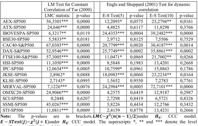
Previous studies have adopted a constant conditional correlation assumption using the CCC-GARCH approach of Bollerslev (1990). However, Tse (2000) and Engle and Sheppard (2001), among others, have shown that this assumption is too restrictive and may be rejected3.Tse (2000) proposes a test for constant correlations. The testing hypotheses are given by

: ℎ , = ℎ , ℎ , : ℎ , = , ℎ , ℎ ,

(4)

where the conditional variances (ℎ , and ℎ , ) are GARCH(1,1).

The test statistic is a LM statistic which under the null hypothesis is asymptotically ( ( − 1)/2).Engle and Sheppard (2001) propose another test of the constant correlation hypothesis. The following null hypothesis could be tested against the alternative one as follows:

: = ∀

: ℎ( ) = ℎ( ) + ∗ ℎ( ) + ⋯ + ∗ _ℎ( ₎ (5)

The test is easy to implement since implies that coefficients in the regression = ∗+ ∗ _{+ ⋯ +} ∗ ₊ ∗_{are equal to zero, where} ₌ _{ℎ ( ̂} ₋ ₎_. _ℎ _{is like the} _ℎ

operator but it only selects the elements under the main diagonal. ̂ = / _̂ _{is the} _{× 1}_vector

of standardized residuals under the null hypothesis and = (ℎ / , ℎ / , … , ℎ / ).

Therefore, we only estimate by maximum likelihood method the bivariate CCC-GARCH model. Then, we decide on the rejection or acceptance of the null hypothesis. The results of both correlation tests are shown in Table 5. From this table, we find evidence against the constant correlation assumption which is based on the LMC and ES statistics of Tse (2000) and Engle and Sheppard (2001), respectively. Thus, we could reject the null of a constant conditional correlation in favor of a dynamic structure. From this evidence, it is interesting to note that it is important to study the models that allow time-varying correlations. In all cases, the constant correlations assumption must be tested before the empirical multivariate DCC-GARCH models are used for inference and analysis of economic and financial implications.

3

(11)

647

Table 5. Correlation tests

LM Test for Constant Correlation of Tse (2000)

Engle and Sheppard (2001) Test for dynamic correlation

LMC statistic p-value E-S Test(5) p-value E-S Test(10) p-value AEX-SP500 56,3301*** 0,0000 12,2093* 0,0575 23,2794** 0,0161

ATX-SP500 24,646*** 0,0000 4,4825 0,6117 11,8298 0,3766

IBOVESPA-SP500 6,3217** 0,0119 24,4353*** 0,0004 39,2482*** 0,0000

BSE30-SP500 5,5833** 0,0181 2,9712 0,8125 7,5506 0,7529

CAC40-S&P500 67,0303*** 0,0000 20,7799*** 0,0020 30,4187*** 0,0014 DAX-S&P500 52,9546*** 0,0000 25,7749*** 0,0002 35,8861*** 0,0002 FTSE100-S&P500 57,3005*** 0,0000 11,0471* 0,0869 21,7002** 0,0268

HSI-SP500 11,1050*** 0,0009 8,5848 0,1983 13,4201 0,2668

IPC-SP500 12,0654*** 0,0005 10,7599* 0,0961 15,0863 0,1786 JKSE-SP500 2,8962* 0,0888 18,0983*** 0,0060 23,2234** 0,0164

KLSE-SP500 2,7143* 0,0995 1,5652 0,9550 7,2783 0,7761

MERVAL-SP500 7,1226*** 0,0076 24,2984*** 0,0005 72,7101*** 0,0000 OMXC20-SP500 24,9066*** 0,0000 4,2575 0,6419 12,9187 0,2987

SCI-SP500 0,2448 0,6207 2,7298 0,8419 6,5721 0,8326

SSMI-SP500 45,0267*** 0,0000 5,8226 0,4434 12,2766 0,3432

STI-SP500 11,0811*** 0,0009 2,4159 0,8778 13,4231 0,2666 Note: The p-values are in brackets. ~ ( ( − )/ )under : CCC model.

− ( )~ ( + )under : CCC model. The superscripts *, ** and *** denote the level significance at 10%, 5% and 1%, respectively.

4.2. Model specification and estimation results

In this article, we employ a multivariate GARCH model with Dynamic Conditional Correlation (DCC) that allows for time-varying conditional correlation as proposed by Engle (2002).In a first step, we specify the mean equation as follows:

= + + + (6) where

- = ( , , … , )

- = /

- /ℱ ~ (0, )

 : ( × 1)vector of . . errors such that ( ) = 0 and ( ) = .

 ≡ {ℎ } ∀ , = 1,2, … , : ( × )matrix of conditional variances and covariances of conditionally to , ,...

In the mean equation, we include an AR(1) term and the one-day lagged US stock return. The AR(1) term indicates the autocorrelation of stock returns, while the lagged US stock returns account for a global factor. In a second step, we specify a multivariate conditional variance as:

≡ (7) where:

 = { } : ( × ) conditional symmetric correlation4 matrix of at time ;

 = { ℎ } : ( × ) diagonal matrix of conditional standard deviations of at time ; The elements in the diagonal matrix are standard deviations from univariate GARCH models:

ℎ = + ∑ + ∑ ℎ (8)

where > 0; ≥ 0 ; ≥ 0and ∑ + ∑ < 1.

The elements of = are:

[ ] = ℎ ℎ , (9)

As proposed by Engle (2002), the DCC-GARCH model is designed to allow for a two-stage estimation of the conditional covariance matrix . In the first stage, univariate GARCH(1,1) volatility models are fitted for each of the stock return residuals and estimates of ℎ, are obtained. In the

second stage, stock return residuals are transformed by their estimated standard deviations from the

4

(12)

648 first stage as = / ℎ, . Then, the standardized residue is used to estimate the correlation

parameters. The dynamics of the correlation in the standard DCC-GARCH model could be expressed as follows:

= (1 − − ) + + (10) where

- ≥ 0 , ≥ 0 and + < 1;

- = [ , ]: the × time-varying covariance matrix of ;

- = ( ): the × unconditional covariance matrix of .

In addition, , the starting value of ,ought to be positive definite to guarantee to be also positive definite. In a bivariate setting, the conditional covariance could be expressed as follows:

, = 1 − − + , , + , (11)

When specifying the form of the conditional correlation matrix , two requirements have to be considered:

- The conditional covariance matrix5 has to be positive definite;

- All the elements in the conditional correlation matrix have to be equal or less than unity. To ensure both of these requirements in the DCC-GARCH model, the conditional correlation matrix

could be decomposed as follows:

= ∗ / ∗ / (12) where

∗₌ ₍ _{) =}

, ⋯ 0

⋮ ⋱ ⋮

0 ⋯ ,

(13)

=

1 ⋯ ,

⋮ ⋱ ⋮

, ⋯ 1

is a correlation matrix with ones on the diagonal and off-diagonal elements

are less than one in absolute value as long as is positive definite. A typical element of is of the form:

, = ,

, , ∀ , = 1,2, … , ; ≠ (14)

In a bivariate case, the conditional correlation coefficient could be expressed as follows:

, = ,

, , =

( ) _, _, _,

( ) _, _, ( ) _, _, (15)

As noted by Engle (2002), the DCC model could be estimated by using a two-step approach to maximize the log-likelihood function. Let denote the parameters in and the parameters in , then the log-likelihood is:

( , ) = − ∑ ( (2 ) + | | + + − ∑ ( | | + − (16)

The first part of the likelihood function in Eq. (16) is volatility, which is the sum of individual GARCH likelihoods. The log-likelihood function can be maximized in the first stage over the parameters in . Given the estimated parameters in the first stage, the correlation component of the likelihood function in the second stage (the second part of Eq. (16)) could be maximized to estimate correlation coefficients.

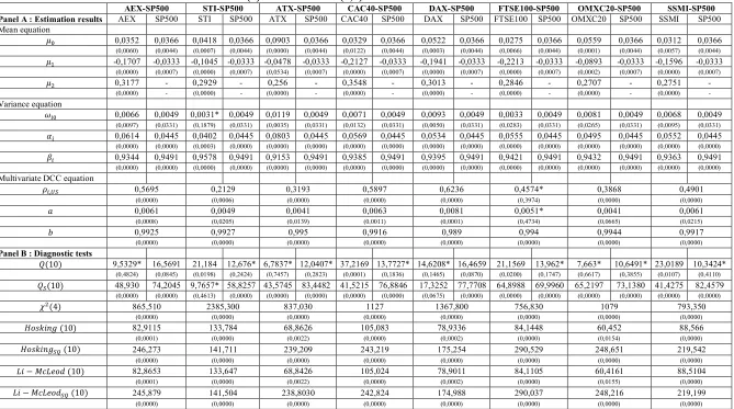
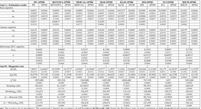
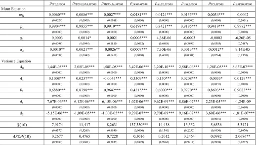
Tables6 and 7 report the estimates of the return and conditional variance equations as well as the DCC parameters. The constant term in the mean equation ( ) is significantly different from zero for the majority of stock markets except for Malaysia and China. With the exception of IPC, JKSE and KLSE returns, the parameter is significantly negative for the remaining stock markets. According to Antoniou et al (2005), the negativity of the AR(1) term in the mean equation is due to the existence of positive feedback trading in developed markets, while the positivity of this parameter in emerging

5

(13)

649 markets is due to price friction or partial adjustment. In addition, the coefficient is statistically positive for the majority of stock markets except for IPC and IBOVESPA returns. The effect of the US stock returns on the returns of those markets is on average highly significant and large in magnitude, ranging from 0.0956 (Argentina) to 0.4249 (Hong Kong).This proves the effect role of the US stock market on the international stock markets. The coefficients for the lagged variance ( ) are positive and statistically significant for all stock markets. Besides, the parameters in the variance equation are significantly different from zero for all stock returns. This justifies the suitability of the GARCH(1,1) specification as the best fitting of the time-varying volatility. Moreover, the quantity

+ is very close to unity, indicating a high short-term persistence of the conditional variance. Therefore, the volatility in the GARCH models display a high persistence.

In Tables 6 and 7, we also report the estimates of the bivariate DCC(1,1) model. The parameters and of the DCC(1,1) model respectively capture the effects of standardized lagged shocks

( ) and the lagged dynamic conditional correlations effects ( ) on current dynamic conditional correlation. The statistical significance of these coefficients in each pair of stock markets indicates the existence of time-varying dynamic correlations. When = 0and = 0, we obtain the Bollerslev’s (1990) Constant Conditional Correlation(CCC) model. Note that the estimated coefficients and are positive and satisfy the inequality + < 1 in each of the pairs of stock markets.As shown in Tables6 and 7, the parameter is statistically significant except for the FTSE-SP500, JKSE-FTSE-SP500, KLSE-FTSE-SP500, HSI-FTSE-SP500, SCI-SP500 and BSE30-SP500 pairs. However, the parameter is highly significant for all stock markets. Note that the significativity of the DCC parameters ( and ) reveals a considerable time-varying comovement and thus a high persistence of the conditional correlation. The sum of these parameters is close to unity and range between 0.8788 (USA-Indonesia) and 0.9995 (USA-India). This implies that the volatility displays a highly persistent fashion. Since + < 1, the dynamic correlations revolve around a constant level and the dynamic process appears to be mean reverting. We also note the existence of 16 unconditional correlations pairs of the standardized innovations from the estimated univariate GARCH models. The values of these correlations vary between 0.0687 (USA-China) and 0.6882 (USA-Mexico).

The multivariate DCC-GARCH model of Engle (2002) has some advantages. First, it allows obtaining all possible pair-wise conditional correlation coefficients for the index returns in the sample. Second, it’s possible to investigate their behavior during periods of particular interest, such as periods of 2007-2010 financial crisis. Third, we were able to look at possible financial contagion effects between the US and international stock markets which have been affected by the recent 2007-2010 financial crisis.

Boyer et al. (2006) show that contagion can either be investor induced through portfolio rebalancing or fundamental based. The latter can be associated to the interdependence phenomenon (Forbes and Rigobon, 2002), while the former case is described in behavioral finance literature as herding (i.e. continued high correlation). Hirshleifer and Teoh (2003) argue that the herding behavior can occur since investors are following other investors and characterize it as convergence of behaviors. The result of such herding behavior is a group of investors trading in the same direction over a period of time. Using the dynamic conditional correlation measure, Bekaert and Harvey (2000), Corsetti et al. (2005), Boyer et al. (2006), Chiang et al. (2007), Jeon and Moffett (2010) and Syllignakis and Kouretas (2011), among others, investigate potential herding behavior in financial markets during crises periods.

(14)

650 diagnostic tests allow detecting serial correlation on the standardized and squared standardized residuals and thus the evidence of the ARCH effects.

4.3. Statistical analysis of conditional correlation coefficients

In Table 8, we report some descriptive statistics of the conditional correlations of the sixteen pair-wise stock markets under study. All the pair-pair-wise stock markets display positive conditional correlation. The highest conditional correlation mean value (0.6777) is between Mexico and USA, while China and USA exhibit the lowest conditional correlation mean value (0.0643). It should be noted that higher conditional correlations values are associated to extreme movements. For the majority of stock markets, the conditional correlations exhibit high standard deviations. The skewness, Excess kurtosis and the Jarque-Bera test statistics indicate that all the pair-wise DCCs exhibit significant departure from the normal distribution. The kurtosis statistic reveals that the DCCs time series are highly leptokurtic. This could be attributed to the existence of some extreme events in the DCCs behavior over the sample period. This observation is supported by Figure 2 prescribing the pair-wise conditional correlations dynamics. The figure shows the estimated dynamic correlation coefficients (DCC) for each pair of the financial contagion source (USA) and target country.

In Figure 2, we report the estimated dynamic conditional correlations using the bivariate DCC(1,1)-GARCH(1,1) modeling framework. By examining the evolution of these correlations, we note the existence of various tendencies. This suggests that interpretations based on the constant correlations assumption may be misleading and erroneous. The graphical analysis of the correlation coefficients leads to interesting observations. First, we note that whatever the considered couple of stock indices returns, there exist parcels of high and low correlations. Indeed, we observe that correlation between stock market returns and the US stock return range from a maximum value of (0.8) and a minimum value of (-0.05). Moreover, there exist peaks and troughs that justify the dynamic nature of the conditional cross-correlations. For example, there are peaks and troughs in the correlations around the 2007 subprime crisis and 2008 financial crisis periods. In addition, we note the existence of a sudden drop in cross-correlations followed by a sharp rise and this in the beginning of the considered study period. The magnitude of these changes appears to be particularly important for the stock markets. These high correlation levels obviously reflect the increasing integration of these markets.

(15)

651

Table 6. Estimation results from the bivariate AR(1)-DCC-GARCH(1,1) model.

AEX-SP500 STI-SP500 ATX-SP500 CAC40-SP500 DAX-SP500 FTSE100-SP500 OMXC20-SP500 SSMI-SP500

Panel A : Estimation results AEX SP500 STI SP500 ATX SP500 CAC40 SP500 DAX SP500 FTSE100 SP500 OMXC20 SP500 SSMI SP500 Mean equation

0,0352 0,0366 0,0418 0,0366 0,0903 0,0366 0,0329 0,0366 0,0522 0,0366 0,0275 0,0366 0,0559 0,0366 0,0312 0,0366 (0,0060) (0,0044) (0,0007) (0,0044) (0,0000) (0,0044) (0,0122) (0,0044) (0,0003) (0,0044) (0,0066) (0,0044) (0,0001) (0,0044) (0,0057) (0,0044) -0,1707 -0,0333 -0,1045 -0,0333 -0,0478 -0,0333 -0,2127 -0,0333 -0,1941 -0,0333 -0,2213 -0,0333 -0,0893 -0,0333 -0,1596 -0,0333

(0,0000) (0,0007) (0,0000) (0,0007) (0,0534) (0,0007) (0,0000) (0,0007) (0,0000) (0,0007) (0,0000) (0,0007) (0,0002) (0,0007) (0,0000) (0,0007)

0,3177 - 0,2929 - 0,256 - 0,3548 - 0,3013 - 0,2846 - 0,2707 - 0,2751 -

(0,0000) - (0,0000) - (0,0000) - (0,0000) - (0,0000) - (0,0000) - (0,0000) - (0,0000) -

Variance equation

0,0066 0,0049 0,0031* 0,0049 0,0119 0,0049 0,0071 0,0049 0,0093 0,0049 0,0033 0,0049 0,0081 0,0049 0,0068 0,0049 (0,0097) (0,0331) (0,1879) (0,0331) (0,0035) (0,0331) (0,0132) (0,0331) (0,0050) (0,0331) (0,0283) (0,0331) (0,0265) (0,0331) (0,0095) (0,0331) 0,0614 0,0445 0,0402 0,0445 0,0803 0,0445 0,0569 0,0445 0,0534 0,0445 0,0555 0,0445 0,0495 0,0445 0,0552 0,0445 (0,0000) (0,0000) (0,0003) (0,0000) (0,0000) (0,0000) (0,0000) (0,0000) (0,0000) (0,0000) (0,0000) (0,0000) (0,0000) (0,0000) (0,0000) (0,0000) 0,9344 0,9491 0,9578 0,9491 0,9153 0,9491 0,9385 0,9491 0,9395 0,9491 0,9421 0,9491 0,9432 0,9491 0,9363 0,9491 (0,0000) (0,0000) (0,0000) (0,0000) (0,0000) (0,0000) (0,0000) (0,0000) (0,0000) (0,0000) (0,0000) (0,0000) (0,0000) (0,0000) (0,0000) (0,0000) Multivariate DCC equation

, 0,5695 0,2129 0,3193 0,5897 0,6236 0,4574* 0,3868 0,4901

(0,0000) (0,0006) (0,0000) (0,0000) (0,0000) (0,3974) (0,0000) (0,0000)

0,0061 0,0049 0,0041 0,0063 0,0081 0,0051* 0,0041 0,0061

(0,0008) (0,0205) (0,0139) (0,0011) (0,0001) (0,4734) (0,0665) (0,0215)

0,9925 0,9927 0,995 0,9916 0,989 0,994 0,9944 0,9917

(0,0000) (0,0000) (0,0000) (0,0000) (0,0000) (0,0000) (0,0000) (0,0000)

Panel B : Diagnostic tests

(10) 9,5329* 16,5691 21,184 12,676* 6,7837* 12,0407* 37,2169 13,7727* 14,6208* 16,4659 21,1569 13,962* 7,663* 10,6491* 23,0189 10,3424* (0,4824) (0,0845) (0,0198) (0,2424) (0,7457) (0,2823) (0,0001) (0,1836) (0,1465) (0,0870) (0,0200) (0,1747) (0,6617) (0,3855) (0,0107) (0,4110) (10) 48,930 74,2045 9,7657* 58,8257 43,5745 83,4482 41,5215 76,8846 17,3252 77,7708 64,8988 69,9960 65,2197 73,1380 41,4275 82,4579

(0,0000) (0,0000) (0,4613) (0,0000) (0,0000) (0,0000) (0,0000) (0,0000) (0,0675) (0,0000) (0,0000) (0,0000) (0,0000) (0,0000) (0,0000) (0,0000)

(4) 865,510 2385,300 837,030 1127 1367,800 756,830 1079 793,350

(0,0000) (0,0000) (0,0000) (0,0000) (0,0000) (0,0000) (0,0000) (0,0000)

(10) 82,9115 133,784 68,8626 105,083 78,9336 84,1448 60,452 88,566

(0,0001) (0,0000) (0,0022) (0,0000) (0,0002) (0,0000) (0,0154) (0,0000)

(10) 246,273 141,711 239,209 243,219 175,254 290,529 248,651 219,542

(0,0000) (0,0000) (0,0000) (0,0000) (0,0000) (0,0000) (0,0000) (0,0000)

− (10) 82,8653 133,647 68,8426 105,024 78,9011 84,1105 60,4161 88,5104

(0,0001) (0,0000) (0,0022) (0,0000) (0,0002) (0,0000) (0,0155) (0,0000)

− (10) 245,879 141,504 238,8030 242,824 174,988 290,037 248,216 219,199

(0,0000) (0,0000) (0,0000) (0,0000) (0,0000) (0,0000) (0,0000) (0,0000)

(16)

652

Table 7. Estimation results from the bivariate AR(1)-DCC-GARCH(1,1) model (continued).

IPC-SP500 BOVESPA-SP500 MERVAL-SP500 JKSE-SP500 KLSE-SP500 HSI-SP500 SCI-SP500 BSE30-SP500

Panel A : Estimation results IPC SP500 BOVESPA SP500 MERVAL SP500 JKSE SP500 KLSE SP500 HSI SP500 SCI SP500 BSE30 SP500 Mean equation

0,0931 0,0366 0,0920 0,0366 0,0889 0,0366 0,1072 0,0366 0,0155* 0,0366 0,0390 0,0366 0,0306* 0,0366 0,1025 0,0366 (0,0000) (0,0044) (0,0001) (0,0044) (0,0004) (0,0044) (0,0000) (0,0044) (0,3073) (0,0044) (0,0096) (0,0044) (0,2082) (0,0044) (0,0000) (0,0044) 0,0342* -0,0333 -0,0411 -0,0333 -0,0517 -0,0333 0,033* -0,0333 0,0198* -0,0333 -0,0866 -0,0333 -0,0516 -0,0333 -0,0273 -0,0333

(0,2613) (0,0007) (0,1449) (0,0007) (0,0423) (0,0007) (0,1492) (0,0007) (0,5749) (0,0007) (0,0000) (0,0007) (0,0104) (0,0007) (0,2241) (0,0007)

0,025* - 0,0467* - 0,0956 - 0,2858 - 0,1553 - 0,4249 - 0,1232 - 0,2313 -

(0,4324) - (0,2689) - (0,0177) - (0,0000) - (0,0000) - (0,0000) - (0,0000) - (0,0000) -

Variance equation

0,0143 0,0049 0,0310 0,0049 0,0566 0,0049 0,0384 0,0049 0,0518 0,0049 0,0056 0,0049 0,0119 0,0049 0,0195 0,0049 (0,0059) (0,0331) (0,0059) (0,0331) (0,0026) (0,0331) (0,0266) (0,0331) (0,0526) (0,0331) (0,0217) (0,0331) (0,0376) (0,0331) (0,0037) (0,0331) 0,0526 0,0445 0,0391 0,0445 0,0559 0,0445 0,0668 0,0445 0,0391 0,0445 0,0417 0,0445 0,0356 0,0445 0,0761 0,0445 (0,0000) (0,0000) (0,0000) (0,0000) (0,0000) (0,0000) (0,0000) (0,0000) (0,0179) (0,0000) (0,0000) (0,0000) (0,0000) (0,0000) (0,0000) (0,0000) 0,9356 0,9491 0,9462 0,9491 0,9198 0,9491 0,9062 0,9491 0,8952 0,9491 0,9540 0,9491 0,9593 0,9491 0,9167 0,9491 (0,0000) (0,0000) (0,0000) (0,0000) (0,0000) (0,0000) (0,0000) (0,0000) (0,0000) (0,0000) (0,0000) (0,0000) (0,0000) (0,0000) (0,0000) (0,0000) Multivariate DCC equation

, 0,6882 0,6669 0,5332 0,1346 0,0889 0,1818 0,0687 0,1702

(0,0000) (0,0000) (0,0000) (0,0000) (0,0055) (0,0000) (0,0237) (0,7472)

0,0099 0,0164 0,0187 0,0068* 0,0043* 0,0152* 0,0092* 0,0031*

(0,0660) (0,0000) (0,0003) (0,4180) (0,3318) (0,4877) (0,1235) (0,1641)

0,9836 0,9773 0,9775 0,8720 0,9730 0,8990 0,9398 0,9964

(0,0000) (0,0000) (0,0000) (0,0000) (0,0000) (0,0000) (0,0000) (0,0000)

Panel B : Diagnostic tests

(10) 7,9691* 14,6463* 10,5594* 10,3573* 8,4584* 10,3044* 15,877* 11,495* 17,9281 10,6809* 19,6384 12,5186* 24,179 10,5455* 14,6684* 13,3338* (0,6319) (0,1455) (0,3929) (0,4097) (0,5842) (0,4142) (0,1032) (0,3203) (0,0562) (0,3829) (0,0329) (0,2518) (0,0071) (0,3940) (0,1446) (0,2056) (10) 54,8794 79,7183 53,4361 51,5548 59,3017 83,3945 45,1833 60,0457 5,4831 62,4020 51,0106 59,9962 31,7035 66,2709 37,4773 62,748 (0,0000) (0,0000) (0,0000) (0,0000) (0,0000) (0,0000) (0,0000) (0,0000) (0,8567) (0,0000) (0,0000) (0,0000) (0,0004) (0,0000) (0,0000) (0,0000)

(4) 1059,800 905,230 1269,800 1489,300 6084,600 915,330 1425 1492,600

(0,0000) (0,0000) (0,0000) (0,0000) (0,0000) (0,0000) (0,0000) (0,0000)

(10) 60,1651 41,1316* 42,5622* 103,505 77,4217 98,3913 64,0343 108,619

(0,0163) (0,3774) (0,3204) (0,0000) (0,0002) (0,0000) (0,0070) (0,0000)

(10) 214,073 195,915 196,935 239,307 119,118 258,050 150,272 194,431

(0,0000) (0,0000) (0,0000) (0,0000) (0,0000) (0,0000) (0,0000) (0,0000)

− (10) 60,1482 41,1334* 42,5671* 103,410 77,3869 98,3334 63,9858 108,557

(0,0164) (0,3773) (0,3202) (0,0000) (0,0002) (0,0000) (0,0070) (0,0000)

− (10) 213,751 195,593 196,610 238,874 119,015 257,595 150,012 194,122

(0,0000) (0,0000) (0,0000) (0,0000) (0,0000) (0,0000) (0,0000) (0,0000)

Notes: The p-values are in parentheses. The superscript * denotes the acceptance of null hypothesis. ( )and ( ) denote the Box-Pierce tests of serial correlation on both standardized and squared standardized residuals. ( )test statistic refers to the vector normality test. ( )and ( ) denote the Hosking's Multivariate Portmanteau Statistics on both Standardized and squared standardized Residuals.

(17)

653

Table 8. Statistical properties of the Multivariate GARCH-DCC’s

Pair-wise stock markets Mean Std.dev Min Max Skewness Excess Kurtosis Jarque-Bera statistic p-value statistic p-value statistic p-value Netherlands-USA 0,5406 0,0958 0,3403 0,7170 -0,0758* 0,0941 -1,0345*** 0,0000 133,090*** 0,0000 Singapore-USA 0,1959 0,0641 0,0481 0,3234 -0,1513*** 0,0008 -0,9525*** 0,0000 121,610*** 0,0000 Austria-USA 0,3660 0,1103 0,2167 0,6218 0,7102*** 0,0000 -0,6785*** 0,0000 301,660*** 0,0000 France-USA 0,5691 0,0343 0,3022 0,7989 -1,0731*** 0,0000 7,7034*** 0,0000 7785,700*** 0,0000 Germany-USA 0,5822 0,0953 0,3835 0,7546 -0,1819*** 0,0001 -1,2132*** 0,0000 195,310*** 0,0000 UK-USA 0,5046 0,1091 0,3096 0,7257 0,3070*** 0,0000 -0,8321*** 0,0000 130,200*** 0,0000 Denmark-USA 0,3650 0,0849 0,1888 0,5090 -0,0362*** 0,4240 -1,2731*** 0,0000 197,980*** 0,0000 Switzerland-USA 0,4604 0,1036 0,2269 0,6425 -0,1475*** 0,0011 -0,9867*** 0,0000 129,130*** 0,0000 Mexico-USA 0,6777 0,0736 0,4337 0,8160 -0,3507*** 0,0000 -0,2922*** 0,0012 70,277*** 0,0000 Brazil-USA 0,6480 0,1079 0,3427 0,8381 -0,2839*** 0,0000 -0,7136*** 0,0000 101,250*** 0,0000 Argentina-USA 0,4843 0,2041 -0,0305 0,8333 -0,3296*** 0,0000 -0,8380*** 0,0000 138,390*** 0,0000 Indonesia-USA 0,1277 0,0067 0,0932 0,1655 0,3843*** 0,0000 3,3159*** 0,0000 1410,600*** 0,0000 Malaysia-USA 0,0788 0,0002 0,0764 0,0810 -1,0837*** 0,0000 30,4250*** 0,0000 1,13E+05*** 0,0000 Hong Kong-USA 0,1687 0,0228 0,0819 0,2707 0,2036*** 0,0000 1,1628*** 0,0000 184,800*** 0,0000 China-USA 0,0643 0,0399 -0,0437 0,3657 1,3601*** 0,0000 6,6904*** 0,0000 6350,600*** 0,0000 India-USA 0,1583 0,0844 0,0455 0,3249 0,8049*** 0,0000 -0,9406*** 0,0000 423,200*** 0,0000 Note: The superscripts *, ** and *** denote the level significance at 10%, 5% and 1%, respectively.

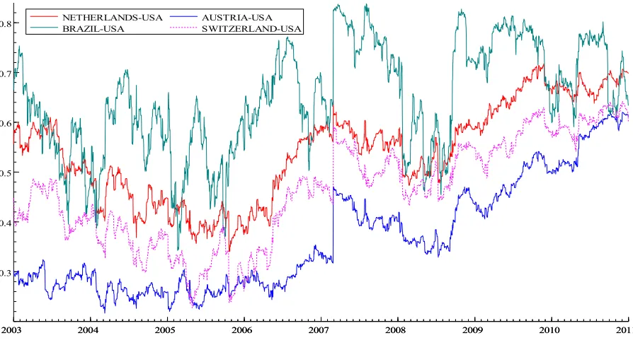
As shown in Figure 2, the pair-wise conditional-correlation coefficients between the US stock return and the remaining stock returns were seen to be persistently higher and more volatile in the second phase of the 2007-2010 financial crisis (09/15/2008 to 12/31/2010). Indeed, the conditional correlations are extremely volatile with some jumps over time. This observation is in line with the stochastic properties of the Multivariate DCC-GARCH model reported in Tables 6 and 7. This leads to two important implications from the investor’s perspective. First, a higher level of correlation implies that the benefit from market-portfolio diversification diminishes, since holding a portfolio with diverse country stocks is subject to systematic risk. Second, a higher volatility of the correlation coefficients suggests that the stability of the correlation is less reliable, casting some doubts on using the estimated correlation coefficient in guiding portfolio decisions. For these reasons, we need to look into the time-series behavior of correlation coefficients and sort out the impacts of external shocks on their movements and variability.

Figure 2. Dynamic Conditional Correlations between the US and Stock Markets-Full Sample

2003 2004 2005 2006 2007 2008 2009 2010 2011

0.3 0.4 0.5 0.6 0.7

0.8 NETHERLANDS-USA

BRAZIL-USA

(18)

654

2003 2004 2005 2006 2007 2008 2009 2010 2011

0.2 0.3 0.4 0.5 0.6 0.7 0.8

FRANCE-USA United Kingdom-USA

GERMANY-USA DENMARK-USA

2003 2004 2005 2006 2007 2008 2009 2010 2011

0.0 0.1 0.2 0.3 0.4 0.5 0.6 0.7

0.8 INDIA-USA

ARGENTINA-USA

(19)

655 In what follows, we examine the DCC’s shifts behavior around the 2007-2010 financial crisis. Mainly, we investigate the effects of the 2007-2010 financial crisis events on the dynamic conditional correlations. Then, we provide supplementary insights into the potential explanatory factors that drive the stock market correlations. In a first stage, we estimate the impact of external shocks on the dynamic conditional correlations feature. The influence of the 2007-2010 financial crisis events on the conditional correlation coefficients is of particular interest. Indeed, the need and the benefits arising from the application of portfolio diversification techniques are higher in periods of market turbulence. Using two dummy variables for different sub-samples allows us to investigate the dynamic feature of the correlation coefficients changes associated with different phases of the 2007-2010 financial crisis. Following Chiang et al. (2007), we regress the time-varying correlation model as follows:

, = + ∑ , + ∑ , + , (17)

where , is the pair-wise conditional correlation coefficient between the stock return( )of the US and

the stock returns ( )of Netherlands, Austria, Brazil, Argentina, India, France, Germany, United Kingdom, Hong Kong, Mexico, Indonesia, Malaysia, Denmark, China, Singapore and Switzerland.

, is a dummy variable for the first phase of the crisis (08/01/2007 to 09/14/2008). , is a

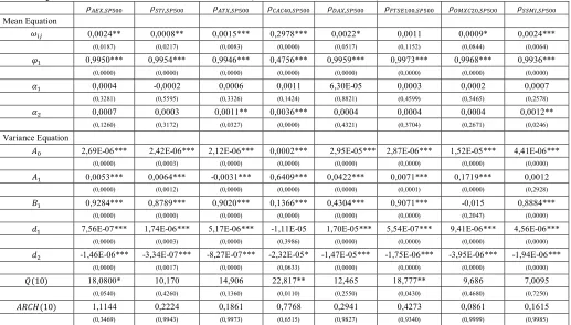
dummy variable for the second phase of the crisis (09/15/2008 to 12/31/2010). Thus, the 2007 subprime crisis is the first phase of the 2007-2010 financial crisis with 411 observations, while the 2008 financial crisis is the second one with 838 observations. The value of the dummy variables is set equal to unity for the crises periods and zero otherwise. We use the AIC and SBIC criterion to determine the lag length in Eq. (17).From the descriptive statistics of the time-varying correlation series, we find significant heteroskedasticity in all cases. Therefore, the conditional variance equation is assumed to follow a GARCH(1,1) specification including two dummy variables, _, ( = 1,2):

ℎ, = + + ℎ, + ∑ , (18)

with > 0, ≥ 0, ≥ 0 and + < 1.

The estimation results of the GARCH(1,1) model for time-varying correlations are reported in Tables 9 and 10. In the mean equation, the coefficient is only statistically significant for Brazil-USA and Indonesia-Brazil-USA pair of countries. This indicates that the correlation during the first phase of the crisis is significantly different from that of the pre-crisis period. This finding indicates existence of contagion phenomenon between the US, Brazilian and Indonesian stock markets. For the remaining

2003 2004 2005 2006 2007 2008 2009 2010 2011

0.00 0.05 0.10 0.15 0.20 0.25 0.30

0.35 INDONESIA-USA SINGAPORE-USA

(20)

656 pairs of countries, the correlations during the early phase of the 2007-2010 financial crisis are not significantly different from that before-crisis period. This may reveal the fact that there exists a drop in the conditional correlation coefficients at the beginning of the 2007-2010 financial crisis. This drop could be explained by the fact that the news may be considered as a single-country case and the crisis signal has not been fully recognized.

Nevertheless, as time passes and investors steadily learn the negative news influencing stock market development, they begin to follow the throngs [see Chiang et al. (2007)]. This means that they start to mimic more reputable investors. Since the risk of investment losses becomes prevalent, the dispersed stock market behavior progressively converges as information accumulates, leading to more uniform behavior and producing a high correlation. Indeed, the correlation turns out to be more significant when any information or news about one stock market is interpreted as information for the whole region.

In the second phase of the 2007-2010 financial crisis, the parameters are significantly positive for Austria-USA, France-USA, Switzerland-USA, Mexico-USA, Brazil-USA, Argentina-USA, Indonesia-USA, Hong Kong-USA and China-USA stock market pairs. Thus, the high correlation with those markets is seen in the second phase of the crisis as reflected by the significant increase in the coefficients on in the mean equation.

Figure 2 shows the co-movement paths and supports the herding behavior assumption in the second phase of the 2007-2010 financial crises. For the remaining countries, investors are more rational in analyzing the fundamentals of the individual stock markets rather than adopting the herding behavior after others. The high correlation between the US and some stock markets in the second phase of the 2007-2010 financial crises (after the 2007 subprime crisis) is consistent with the wake-up call6 hypothesis of Goldstein (1998).

The estimates of the shock-squared errors ( ) and lagged variance ( ) are highly significant except for Switzerland-USA and Denmark-USA cases, exhibiting a clustering phenomenon. Moreover, the parameters are positive and highly significant except for France and India cases, respectively. These findings indicate more volatility changes in the conditional correlation coefficients around the 2007-2010 financial crisis. Finally, during the 2008-2010 financial crisis, the conditional correlation coefficients given by the estimates of the _, in the variance equation (i.e. ) were positive and increased significantly only for Indonesia-USA, Malaysia-USA, Hong Kong-USA and China-USA stock market pairs. However, the coefficient seems to be significantly negative for the remaining market pairs.

The second dummy variable seems to have positive and significant impact on the conditional correlation mean equation for the conditional correlations only between the US and Hong Kong, the US and Indonesia, the US and Malaysia, and the US and China. Hence, the recent 2007-2010 financial crisis have significantly increased correlations (i.e. contagion) between the US and these countries. This suggests that when the crisis occurred in the US stock market, the correlation have varied intensely and this variability seems to be persistent over time. Consequently, the estimates and statistical inference of risk based on constant correlation models could be spurious. Chiang et al. (2007) argue that when any public news about one country is interpreted as information for the entire region, the correlation becomes more significant. Further, our empirical results are consistent with our preliminary analysis of the DCC behavior over time (Figure 2). Moreover, the finding for the Hong Kong-USA, Indonesia-USA, Malaysia-USA and China-USA cases provides support for the evidence of Herding behavior (i.e. continued high correlation) during the 2008-2010 stock market crash. Therefore, the extent of the effect of the 2008-2010 financial crises on the conditional correlation coefficient is revealed by the magnitude of the estimated parameters, which were significantly higher than those of the 2007-2008 subprime crisis.

Our empirical results support those of Chiang et al. (2007) and Syllignakis and Kouretas (2011) by providing substantial evidence in favor of contagion effects due to herding behavior in the emerging financial markets during the 2008-2010 stock market crash. Indeed, in times of severe stress that were

6

(21)

657 experienced in 2008-2010, disparate markets will tumble together as investors scramble to sell their assets and move into cash (see Syllignakis and Kouretas, 2011).

The empirical analysis of the pattern of the time-varying correlation coefficients, during the 2007-2010 financial crisis periods, provides evidence in favor of contagion effects due to herding behavior in international emerging stock markets. Our empirical findings seem to be important to researchers and practitioners and especially to active investors and portfolio managers who include in their portfolios equities from the emerging stock markets. Indeed, the high correlation coefficients, during crises periods, imply that the benefit from international diversification, by holding a portfolio consisting of diverse stocks from the contagious stock markets, decline. Furthermore, the statistical inference of high volatility of conditional correlation coefficients during the 2007-2010 financial crisis periods may mislead the managers’ portfolio decisions. Moreover, our findings are important for policy makers in emerging markets since the instability through financial contagion influences their development. According to Celik (2012), policy makers in emerging countries should seek ways to close the channels of contagion to decrease the instability in emerging countries.

5. Conclusion

This paper is a contribution to the existing empirical literature on financial market contagion. Indeed, it focuses on the increase in the strength of the transmission of the 2007-2010 financial crisis from the US stock market to some major developed and emerging international stock markets. To measure the potential contagion phenomenon, we first use the adjusted correlation approach of Forbes and Rigobon (2002). The main empirical findings of this analysis show the evidence of financial contagion mechanisms in all pairs of stock markets, which departs from the widely cited result of Forbes and Rigobon (2002) of no contagion and only interdependence. Then, we have extended this analysis by taking into account the dynamic feature of the conditional correlation coefficients between stock markets. Mainly, we used the multivariate DCC-GARCH modeling structure to investigate the existence of increased correlation patterns during crisis periods as well as the potential financial contagion effects from the US stock market to some developed and emerging stock markets. Our results indicate the existence of financial contagion effects due to herding behavior in the emerging stock markets, particularly around the 2007-2010 financial crisis. We find statistically highly significant effect on the dynamic conditional correlations during the crisis periods. Moreover, we provide further evidence in favor of financial contagion effects that take place early in the 2007-2010 financial crises as well as the herding behavior in the latter stages of the crisis.

(22)

658

Table 9. Tests of significant changes in dynamic conditional correlations between stock market returns during different phases of the 2007-2010 financial crisis (01/01/200331/12/2010).

, , , , , , , ,

Mean Equation

0,0024** 0,0008** 0,0015*** 0,2978*** 0,0022* 0,0011 0,0009* 0,0024***

(0,0187) (0,0217) (0,0083) (0,0000) (0,0517) (0,1152) (0,0844) (0,0064)

0,9950*** 0,9954*** 0,9946*** 0,4756*** 0,9959*** 0,9973*** 0,9968*** 0,9936***

(0,0000) (0,0000) (0,0000) (0,0000) (0,0000) (0,0000) (0,0000) (0,0000)

0,0004 -0,0002 0,0006 0,0011 6,30E-05 0,0003 0,0002 0,0007

(0,3281) (0,5595) (0,3326) (0,1424) (0,8821) (0,4599) (0,5465) (0,2578)

0,0007 0,0003 0,0011** 0,0036*** 0,0004 0,0004 0,0004 0,0012**

(0,1260) (0,3172) (0,0327) (0,0000) (0,4321) (0,3704) (0,2671) (0,0246)

Variance Equation

2,69E-06*** 2,42E-06*** 2,12E-06*** 0,0002*** 2,95E-05*** 2,87E-06*** 1,52E-05*** 4,41E-06***