A Method to Estimate the Effects of Temperature on Cotton Micronaire

MOLECULAR BIOLOGY AND PHYSIOLOGY

A Method to Estimate the Effects of Temperature on Cotton Micronaire

Michael P. Bange*, Greg A. Constable, David B. Johnston, and David Kelly

M.P. Bange*, G.A. Constable, and D.B. Johnson, CSIRO Plant Industry, Locked Bag 59, Narrabri NSW 2390 Australia; D. Kelly, Cotton Seed Distributors, PO Box 1121, Goondiwindi QLD 4390 Australia

*Corresponding author: [email protected] ABSTRACT

Differences in micronaire of cotton fiber can affect grower returns, and influence textile quality. Therefore quantifying those effects that influence micronaire are important in developing management practices to optimise micronaire. This study proposes a method for predicting seasonal crop micronaire. The aim was to quantify the response of micronaire to temperature during boll filling and assess this information’s ability to predict micronaire on an independent dataset. Utilising existing data from sowing time experiments in Australia that spanned three decades, linear responses of micronaire to both daily average and minimum temperatures were developed (r2 =0.68 for

both). These responses coupled with an estimate of temperature during the boll filling period when the majority of bolls were undergoing fiber thickening were able to successfully predict the micronaire on an independent dataset (r2=0.42) despite no adjustment for

other climate and management factors that may influence crop micronaire. The ability to predict temperature effects on micronaire will be useful to assess reasons for seasonal and regional differences in micronaire and assess opportunities to modify micronaire with changes in management practices that influence the timing of boll development.

M

quality trait that reflects a combination of fiber linear density (often referred to as fineness) and fiber maturity (Lord and Heap, 1988). Too high micronaire (> 4.5) may indicate that fiber is

coarse and is undesirable for spinners as it results

in too few fibers in yarn cross section, reducing its strength. Too low micronaire (< 3.8) may mean that fibers are immature, leading to breakages in fibers within the yarn and poor dye uptake during textile processing. As a consequence growers may incur price discounts if micronaire of their cotton falls outside the optimal range (3.8 to 4.5) (Bange

et al., 2009; Bednarz et al., 2002; Gordon and Naylor, 2004).

The degree of fiber thickening or fiber maturity, contributes to differences in micronaire. When comparing fibres of similar perimeter the thicker the layers of cellulose laid down the more mature the fiber, and the higher the micronaire. Since fiber is primarily cellulose any influence on net crop

photosynthesis and carbohydrate production will

have similar influence on fiber thickening.

I t t h e r e f o r e s t a n d s t o r e a s o n t h a t a s

photosynthesis is highly influenced by temperature (El-Sharkawy and Hesketh, 1964); sustained changes in temperature during the fiber thickening period will lead to differences in micronaire. In addition, studies of cotton fiber development

using cultured cotton ovules have shown that cool

temperatures during secondary wall thickening

affected cellulose deposition leading to differences

in fiber weight (Haigler et al., 1990; Roberts et al.,

1992). These studies provided evidence to suggest

that temperature influences on fiber development were also ovule specific during this phase, and was

not entirely dependent on carbohydrate supply;

reinforcing the significant effects of temperature on micronaire.

Many studies have shown that micronaire responds to temperature changes (Gipson and Joham, 1968; Hesketh and Low, 1968; Gipson and Ray, 1970; Wanjura and Baker, 1985; Liakatas et al., 1998; Reddy et al., 1999). Radiation (Pettigrew,

1995; Wang et al., 2006); plant defoliation (Siebert et al., 2006; Bange et al., 2010); water stress

(Hearn, 1994); and competition among bolls

for carbohydrate within the plant (Brook et al., 1992; Pettigrew, 1995), have also been shown to

of the degree of these influences on micronaire is important so that management practices can be developed to optimise micronaire.

Wanjura and Supak (1985) have used this

understanding to predict or analyse consequences

of temperature on micronaire. In this paper an

alternative approach for predicting seasonal crop

micronaire is proposed and tested. The response of micronaire to temperature was developed from micronaire measured from sowing time studies, and the use of a new approach to estimate the temperature during the fiber thickening phase of a crop’s boll filling period was used. The ability of this approach to predict micronaire was tested

against an independent dataset. This approach can be utilised to predict or analyse the effects on seasonal

temperatures on micronaire such that management decisions may be refined to improve micronaire.

MATERIALS AND METHODS

Estimating temperature effects on micronaire.

Fiber development for an individual boll occurs between flowering and boll maturity (defined as a

cracked boll). This period is often referred to as the

boll period. Fiber development during the boll period can be divided into three phases: fiber elongation, secondary wall thickening, and maturation (Ryser,

1999). For Gossypium hirsutum, fiber elongation

occurs over approximately 20 d (Gipson and Joham, 1968; Gipson and Ray, 1969; Benedict et al., 1973; Meinert and Delmer, 1977), but this period can vary with temperature (Gipson and Joham, 1968, 1969;

Gipson and Ray, 1969). Fiber thickening leading to

differences in micronaire occurs over a period of approximately 40 d (Shubert et al., 1973; Benedict et al., 1973) following fiber elongation and similarly varies with temperature (Gipson and Joham, 1968).

To estimate the period of fiber elongation and fiber thickening leading to differences in micronaire, thermal time of an average boll period of 68 d (750 day degrees (DD)) (Constable, 1991; Hearn and Constable, 1984; Constable and Shaw, 1988) was divided proportionally using 20 d for fiber elongation and the following 40 d for fiber thickening. This equates to a 220 DD for the fiber elongation period and 440 DD for the fiber thickening phase. The remaining time is considered the fiber maturation phase in which the fibers dry, causing the vacuole (lumen) to collapse and the fiber to die.

Fiber quality data for these studies came from multisite experiments over a number of seasons. In order to determine any relationship between micronaire and temperature, it was necessary to retrospectively estimate development as above. Micronaire was compared with temperatures during mid boll fill, specifically from about 1200 to 1440 DD from sowing. These dates were chosen to represent the stage when the majority of bolls in a crop were estimated to be at the fiber thickening stage. Some earlier bolls would not

have reached fiber thickening at 1200 DD and

some later bolls may still be thickening after 1440 DD. Those points in development were chosen

as follows:

The start of flowering was estimated as 777

DD (Constable, 1991) after sowing. Cold shocks

delay flowering when minimum temperature

reaches or falls below 11oC (Hearn and Constable, 1984). It was assumed that these crops required

ten fruiting nodes to contribute to the majority of yield (Constable, 1991). The mid point of

flowering was therefore five nodes after first flower (at 42 DD per node, or 210 DD). Since fiber elongation occurs in the first 220 DD after flowering, the point when all bolls have reached the fiber thickening stage is 777+210+220 = 1197

DD. Fiber thickening is complete for the first bolls when 777+660 = 1437 DD. From that point, successive bolls are mature, and the period when

all bolls are thickening ceases. Daily average and

minimum temperature are then calculated for this

fiber thickening period.

Day degrees (DD) were derived using a base

temperature of 12°C (Constable and Shaw, 1988):

(

) (

)

[

]

degrees

Day = Tmax− + Tmin− (1)

where Tmax and Tmin are daily maximum and

minimum temperatures respectively. When Tmin <

12°C, Tmin =12. (or (Tmin – 12) > 0.0).

Response of micronaire to temperature.

To develop a relationship to temperature during the boll filling period of crop development measurements from sowing time experiments

were utilised. These studies were grown with full

nutrition and water requirements with sowing time, season, and location, all contributing to differences in temperature experienced by the crop during boll filling. Details of each experiment are

For each treatment of each experiment, daily average and minimum temperature during boll development were derived using the methodology described above. For the Narrabri location, climate data was obtained using records from the Australian

Cotton Research Institute. For other locations,

climate data was obtained from records from the nearest major town to the experiment site using the

SILO patched point dataset (Jeffrey et al., 2001)

that uses Australian Bureau of Meteorology official weather stations. Where experiments recorded the date on which first flower occurred, this information was used to initiate the time when temperature was estimated, otherwise timing of first flower was

predicted, as described above.

Micronaire for each sowing treatment (averaged across cultivars) for each experiment was then

regressed with the derived daily average and

minimum temperature. Regression analysis was used

to fit both linear and quadratic functions (Sigma Plot

ver. 11, Systat Software, Inc., San Jose, California).

Relative improvement of the quadratic response

over the linear response was tested using F-tests

based on residual means squares (RMS) accounting for differences in the function’s degrees of freedom (Cousens, 1985).

Predicting micronaire from temperature.For

validation purposes micronaire was compiled for a number of commercial cultivars grown in cultivar

evaluation studies undertaken by Cotton Seed Distributors (CSD). The cultivars were grown across a range of sites in existing cotton regions in Australia

from southern New South Wales (NSW) to central Queensland (Qld) in crops sown from 2000 to 2007. Micronaire from four CSIRO cultivars was compiled; Sicot 71, Sicot 71B, Sicot 71BR, and

Sicot 71 BRF. These were chosen because they were

the most widely grown commercially across regions

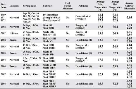
Table 1. Details of sowing time experiments used to generate the responses of micronaire to temperature. Origin of all cultivars are from CSIRO† Australia unless specified. Average cultivar micronaire values were measured by CSIRO’s cotton breeding program long term dataset. With the exception of the study by Constable et al. where micronaire was measured using an areolometer, all other micronaire measurements were measured using a High Volume Instrument (HVI). The highest and lowest daily average minimum and maximum temperatures recorded for each experiment are also shown. These temperatures were estimated using the approach proposed in this paper.

Year

Sown Location Sowing dates Cultivars

First Flower Measured

Published

Average Min. Temperature

(˚C)

Average Max. Temperature

(˚C)

Average Cultivar Micronaire

1969 1971

1972 Narrabri

Sep. 30, Oct. 10, Oct. 20, Oct. 30, Nov. 10, Nov. 20, Nov. 30

DP Smoothleaf (Deltapine USA), Short Sympodial No

Constable et al. (1976) (1)‡

13.4 13.4 17.5

32.6 30.1

32.8 3.95

2002 Narrabri 24 Sep., 15 Oct., _{11 Nov.} Sicot 189_{Sicot 289B} Yes Bange et al. _{(2008) (2)} 17.8 36.4 4.19_4.49

2002 Hillston 27 Sep., 24 Oct., _{27 Nov.} Sicala S40i_{Siokra V-16i} No Bange et al. _{(2004) (3)} 15.0 34.9 4.16_3.97

2002 Breeza 25 Sep., 16 Oct., _{18 Nov.} Siokra S101i_{Sicala V3i} Yes Unpublished (4) 12.6 33.5 3.97_3.98

2003 Narrabri 13 Oct., 5 Nov., _{28 Nov.} Sicot 189R_{Sicot 289BR} Yes Bange et al. _{(2008) (5)} 15.7 34.9 4.04_4.29

2003 Breeza 26 Sep., 14 Oct., _{4 Nov.} Sicala 43_{Sicala 43B} No Unpublished (6) 17.8 32.9 4.26_4.30

2004 Narrabri 6 Oct., 22 Oct., 28 _Nov. Sicot 189R_{Sicot 289BR} Yes Bange et al. _{(2008) (7)} 17.9 34.1 4.04_4.29

2004 Breeza 28 Sep., 14 Oct., _{27 Oct.} Sicala V3BR_{Sicala 60BR} Yes Unpublished (8) 14.5 33.8 4.16_4.47

2007 Narrabri 16 Oct., 13 Nov. Sicot 71BRSicot 70BRF

Sicot F1BRF Yes Unpublished (9) 12.9 30.4

4.50 4.13 4.37

2008 Narrabri 16 Oct., 14 Nov. Sicot 71BRSicot 70BRF

Sicot F1BRF Yes Unpublished (10) 15.7 32.8

4.50 4.13 4.37

† CSIRO (Commonwealth Scientific and Industrial Research Organisation Australia).

For each cultivar grown at each site and every year,

temperature during boll development was calculated using the approach for temperature estimation described previously. Climate data was again obtained from the SILO patched point dataset (Jeffrey et al., 2001) for the nearest major weather station (< 50 km). and years. The average micronaire of these cultivars

obtained from the CSIRO’s cotton breeding program long-term dataset were: 4.25 for Sicot 71; 4.38 for

Sicot 71B; 4.5 for Sicot 71BR; and 4.13 for Sicot 71BRF. Details of cultivar evaluation data used are

presented in Table 2.

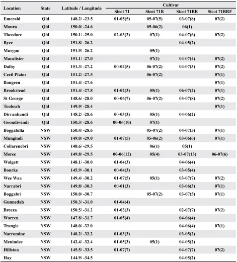
Table 2. Details of information used for micronaire prediction validation from Cotton Seed Distributors (CSD) (Wee Waa, NSW, Australia) cultivar evaluation sites. The range of years in which the cultivar evaluation was conducted and number of sites (in brackets) is shown under respective cultivars. For example 01-05(5) means that the cultivar was evaluated between 2001 and 2005 at five sites in the location specified.

Location State Latitude / Longitude Cultivar

Sicot 71 Sicot 71B Sicot 71BR Sicot 71BRF

Emerald Qld 148.2/ -23.5 01-05(5) 05-07(5) 03-07(8) 07(2)

Moura Qld 150.0/ -24.6 05-06(2) 06(1)

Theodore Qld 150.1/ -25.0 02-03(2) 07(1) 04-07(6) 07(2)

Byee Qld 151.8/ -26.2 04-05(2)

Murgon Qld 151.9/ -26.2 05(1)

Macalister Qld 151.1/ -27.0 07(1) 04-07(4) 07(2)

Dalby Qld 151.3/ -27.2 00-04(5) 06-07(2) 04-07(3) 07(2)

Cecil Plains Qld 151.2/ -27.5 06-07(2) 07(1)

Bongeen Qld 151.4/ -27.6 07(1)

Brookstead Qld 151.4/ -27.8 01-02(3) 05(1) 06-07(2) 07(1)

St George Qld 148.6/ -28.0 00-06(7) 06-07(2) 03-07(8) 07(2)

Toobeah Qld 149.9/ -28.4 07(1)

Dirranbandi Qld 148.2/ -28.6 00-03(3) 05(1) 04-06(2)

Goondiwindi Qld 150.3/ -28.6 00-06(10) 07(1)

Boggabilla NSW 150.4/ -28.6 05-07(2) 04-07(5) 07(1)

Mungindi NSW 149.0/ -29.0 01-07(5) 05-06(2) 03-06(6) 07(1)

Collarenebri NSW 148.6/ -29.5 06(1) 05(1)

Moree NSW 149.8/ -29.5 00-06(12) 05(4) 03-07(13) 06-07(6)

Walgett NSW 148.1/ -30.0 01-04(3) 04-06(4)

Bourke NSW 145.9/ -30.1 00-04(3) 03-05(4)

Wee Waa NSW 149.4/ -30.2 01-07(5) 05(1) 03-07(7) 07(2)

Narrabri NSW 149.8/ -30.3 00-01(3) 03-06(3) 07(1)

Boggabri NSW 150.0/ -30.7 05-07(2) 03-07(5) 07(1)

Gunnedah NSW 150.3/ -31.0 01-04(4)

Breeza NSW 150.5/ -31.2 01-03(3) 02-07(7) 07(2)

Warren NSW 147.8/ -31.7 01-05(4) 04-06(4)

Trangie NSW 148.0/ -32.0 04-06(4) 07(1)

Narromine NSW 148.2/ -32.2 01-03(3) 03-05(2)

Menindee NSW 142.4/ -32.4 01-05(3) 05(1) 04-05(2)

Hillston NSW 145.5/ -33.5 01-07(7) 04-07(7) 07(2)

Sowing time of the CSD cultivar evaluation studies was

the only variable needed to predict daily average and

minimum temperatures. These temperatures were then used to estimate micronaire from the linear responses of micronaire to daily average and minimum temperatures. To assess the performance of this approach to predict micronaire, predicted micronaire was plotted against the measured (observed) micronaire. Accuracy of predictions was quantified using the root mean square deviation (RMSD) between a number

(n) of predicted (P) and observed (O) paired results:

(

)

[

]

/n P O

RMSD= ∑ − _{(Steele and Torrie, 1987)}

RMSD represents a mean weighted difference

between predicted and observed data. The linear regression of predicted versus observed values was used

to quantify bias and the coefficient of determination (r2₎

of this regression described the degree to which the data clustered around a straight line. Linear regression

analyses were conducted using Sigma Plot (ver. 11,

Systat Software, Inc., San Jose, California).

In an attempt to improve accuracy of prediction,

inherent differences in micronaire (Micadj) of the

cultivars were considered. Predicted micronaire

was adjusted using the using the weighted average

(micronaire 4.4) of the cultivars used to generate the micronaire versus temperature responses (Table 1),

and the average micronaire of cultivars (Miccuv) used

in the validation:

(

)

pred

adj Mic Mic

Mic = − 4.4−

where Micpred is the predicted micronaire unadjusted for cultivar differences. The performance of this adjustment was assessed similar to micronaire

predictions unadjusted for cultivar.

RESULTS AND DISCUSSION

Response of micronaire to temperature.

Despite differences in cultivars that spanned

three decades, micronaire was strongly related to average temperature that was estimated using the methodology detailed in this paper. Both the average of the daily minimum and average temperatures experienced during the period of fiber thickening contributing to final micronaire were similar in explaining changes in micronaire across all

sowing times (r2 = 0.68; Table 3; Fig. 1). The use

of quadratic functions slightly improved r2_{, but the}

improvement was not significant (P < 0.05) (Table

3). All experiments fitted the same regression.

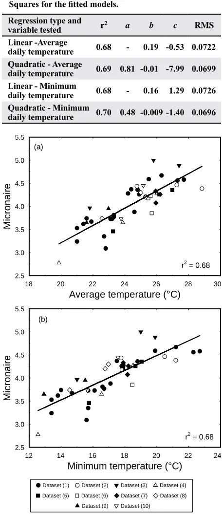
Table 3. Results of regression analyses of micronaire versus daily average temperature and daily minimum temperature averaged for the estimated period of fiber thickening. Data used in this analysis is detailed in Table 1. Linear (y = bx + c) and quadratic regressions (y = ax2 +

bx + c) were tested for each variable. All regressions were highly significant (P < 0.001, n = 46). RMS – Residual Mean Squares for the fitted models.

Regression type and

variable tested r2 a b c RMS Linear -Average

daily temperature 0.68 - 0.19 -0.53 0.0722 Quadratic - Average

daily temperature 0.69 0.81 -0.01 -7.99 0.0699 Linear - Minimum

daily temperature 0.68 - 0.16 1.29 0.0726 Quadratic - Minimum

daily temperature 0.70 0.48 -0.009 -1.40 0.0696

(a)

18 20 22 24 26 28 30

M

ic

ro

n

a

ir

e

M

ic

ro

n

a

ir

e

2.5 3.0 3.5 4.0 4.5 5.0 5.5

r2 = 0.68

(b)

12 14 16 18 20 22 24

2.5 3.0 3.5 4.0 4.5 5.0 5.5

r2 = 0.68

Dataset (1) Dataset (2) Dataset (3) Dataset (4) Dataset (5) Dataset (6) Dataset (7) Dataset (8)

Dataset (9) Dataset (10) Average temperature (°C)

Minimum temperature (°C)

Linear responses of micronaire to temperature

have been previously reported (Gipson and

Joham, 1968; Gipson and Ray, 1970) along with quadratic responses (Hesketh and Low, 1968; Wanjura and Baker, 1985). Reddy et al. (1999) had a linear increase in micronaire to daily average of 30.3°C and a linear decline after this temperature. In this study no significant decline in micronaire was measured when daily average temperature was 28.8°C and daily minimum was 22.7°C. While Wanjura and Baker (1985) used a quadratic response of micronaire to daily average temperature during boll development,

their response showed no substantial decline in

micronaire at 26.6°C. Hesketh and Low (1968) and Reddy et al. (1999) measured significant reductions in micronaire at daily average temperatures during boll filling of 33.5 and 32.3°C respectively. In studies on temperature effects on fiber development in cultured ovules Roberts et

al. (1992) found no decline in cellulose synthesis

with daily temperatures up to 34.0°C.

For micronaire measurements recorded at low temperatures, only studies of Gipson and Joham (1968) (minimum night 8.1°C) and Gipson and Ray (1970) (minimum night 11°C) had lower temperature treatments than those recorded in this study (daily minimum 12.6°C). It is most likely that with more

data collected at higher and lower daily average

temperatures, the response presented here (Fig. 1)

would also be curvilinear.

The degree of change in micronaire with daily minimum temperature in this study (slope 0.16

micronaire units/oC) was greater than measured by

Gipson and Joham (1968) using night temperature. For average daily temperature the slope of the response (0.19) was less than that measured by Wanjura and Baker (1985) (slope 0.41 to 0.56) and similar to that of Reddy et al. (1999) (slope 0.21).

Variations in these responses are expected as these studies differed in the way developing bolls were

exposed to temperature regimes, and how final micronaire values were measured.

This study used daily average and minimum temperatures resulting from changes in sowing time in each experiment, which were applied to micronaire measurements resulting from all bolls harvested from the crop at the end of the season. Controlled environment studies that investigated temperature impacts on micronaire (Gipson and Joham, 1968; Hesketh and Low, 1968; Gipson and

Ray, 1970) maintained minimum and maximum temperatures for longer periods throughout the day using square diurnal temperature control. Therefore impacts of higher and lower temperature extremes on micronaire may be greater resulting in temperature responses having lower slopes or being less responsive to temperature changes. In the Wanjura and Baker (1985) study, daily average temperature for individual cultivars were derived from 10 cohorts of bolls tagged over the duration of crop development. It would therefore be expected that a greater range of temperatures would be recorded during boll development and that the range and differences in micronaire would be larger resulting in more sensitive (greater slopes) micronaire versus temperature responses.

Predicting micronaire from temperature.

Despite taking no account for other factors that

influence micronaire (Constable and Bange, 2007), the methodology that estimated temperature proposed in this study coupled with the micronaire and temperature responses developed (Table 3) were able to predict micronaire well, both on a regionally and temporally diverse dataset (Table 4,

Fig. 2) (r2 0.33 to 0.42). Comparing the ability of daily average and minimum temperature responses to predict micronaire of the CSD data, they were

similar in r2, while the daily average temperature

response had less bias across the micronaire predicted (slope closer to unity). The minimum temperature response did however, slightly increase RMSD by 0.08.

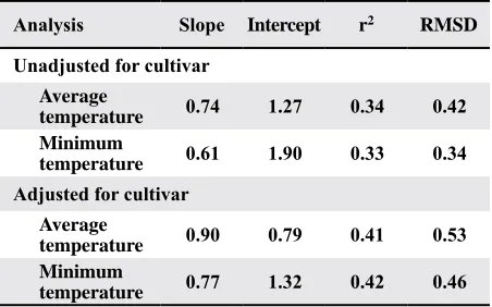
Table 4. The regression coefficient (slope), the coefficient of determination (r2), intercept, and RMSD (root mean

square deviation) for predicted versus observed data for micronaire using average daily and minimum temperature for the estimated period of fiber thickening using Cotton Seed Distributor’s (CSD) dataset. Table includes analysis of predicted micronaire adjusted for individual cultivar differences. (n = 270).

Analysis Slope Intercept r2 _RMSD

Unadjusted for cultivar Average

temperature 0.74 1.27 0.34 0.42

Minimum

temperature 0.61 1.90 0.33 0.34

Adjusted for cultivar Average

temperature 0.90 0.79 0.41 0.53

Minimum

An adjustment in micronaire prediction to

account for inherent cultivar differences reduced the

bias and improved r2 _{but RMSD was only slightly}

increased by 0.1 over the unadjusted prediction (Table 4, Fig. 2). This result was not unexpected

given the limited range of inherent micronaire (Table

1) of the cultivars used for validation (range 0.12). Considering the reasonable ability to predict

micronaire, we see good opportunities to utilise this approach with confidence to explain or predict the effects of seasonal temperature on micronaire of crops.

However, some issues would need consideration before applying this approach more broadly. In addition to extending the temperature range of the micronaire to temperature response mentioned

previously, it would include the need for assessing cultivars that have considerably higher and lower

inherent micronaire than those used in this study. The inherent micronaire difference of cultivars used was narrow (range 0.55) (Table 1). To improve predictions

overall, ongoing research is extending the approach

presented here to target the period of micronaire development to capture the combined effects of water stress, changes in boll load, and temperature.

Application of methodology. Utilising historical

climate data, this approach has been used in the

Australian cotton industry to assess reasons for seasonal

and regional differences in micronaire and assess opportunities to improve micronaire with changes in sowing time (e.g. Fig. 3) (Kelly et al., 2006; 2008). These data demonstrate the importance of avoiding low micronaire as a result of late sowing and also indicates the frequency of high micronaire, which needs to be addressed by crop management and by breeding cultivars with lower linear density. This methodology

will also be able to predict the whole of seasonal effects

on micronaire at the time of harvest aid application and so assist in determining the risks and costs of earlier applications (Wanjura and Newton, 1981). The

opportunity also exists to conduct research to predict the

components of micronaire (linear density and maturity), which may assist in understanding the impact of climate on fiber quality and resulting textile performance.

Fig. 2. Predicted micronaire versus observed micronaire for the fiber thickening period using Cotton Seed Distributor’s (CSD) dataset: (a) micronaire estimated using the linear response of micronaire to daily average temperature (Table 3) un-adjusted for cultivar differences; (b) micronaire estimated using the same response adjusted for cultivar differences. Solid line is the line of best fit. Dashed line is the 1:1 line. (n = 270).

(a)

Observed microniare

2.5 3.0 3.5 4.0 4.5 5.0 5.5 6.0

P

re

di

ct

ed

m

icr

on

ia

re

P

re

di

ct

ed

m

icr

on

ia

re

2.5 3.0 3.5 4.0 4.5 5.0 5.5 6.0

2.5 3.0 3.5 4.0 4.5 5.0 5.5 6.0

(b)

(1:1) (1:1)

r2 _{= 0.41}

r2 _{= 0.34}

2.5 3.0 3.5 4.0 4.5 5.0 5.5 6.0

Day of year (sowing)

240 260 280 300 320 340

M

icr

on

ai

re

3.4 3.6 3.8 4.0 4.2 4.4 4.6 4.8 5.0

Median 80% percentile 20% percentile

CONCLUSION

This study proposed methodology to predict the impacts of temperature on micronaire of cotton crops.

This understanding coupled with knowledge of the degree of the effects of radiation, plant defoliation,

and competition from bolls for carbohydrate within the plant will improve predictions as well as developing management practices to optimise micronaire.

ACKNOWLEDGMENTS

Thanks to Jane Caton for assistance in the collation of data. Dr Robert Long and Mrs Sandra

Williams for helpful discussions about the results.

Thanks to Peter Reid, Dr Warwick Stiller, Dr

Shiming Liu for provision of multisite data and to Kellie Cooper for fibre quality analyses. The Cotton Research and Development Corporation of Australia and the Cotton Catchment Communities Cooperative Research Centre both provided partial financial

support for this work.

REFERENCES

Bange, M.P., S.J. Caton, and S.P. Milroy. 2008. Managing yields of high fruit retention in transgenic cotton (Gossypium hirsutum L.) using sowing date. Aust. J. Agric. Res. 59: 733-741.

Bange, M.P., R.L. Long, G.A. Constable, and S. Gordon. 2010. Minimizing immature fiber and neps in Upland cotton (Gossypium hirsutum L.). Agron. J. 102:781-789. Bange, M.P., E. Brown, J. Caton, and R. Roche. 2004.

Sowing time, variety and temperature effects on crop growth and development in the Hillston region. p. 441-447. In Proc. 12th Aust. Cotton Conf., Gold Coast, Qld, Aust. 12-14 Aug. 2008. The Aust. Cotton Growers

Research Organisation.

Bange, M.P., G.A. Constable, S.G. Gordon, G.R.S. Naylor and M.H.J. Van der Sluijs. 2009. FIBREpak A guide to improving Australian cotton fibre quality. CSIRO and the Cotton Catchment Communities Cooperative Research Centre, Narrabri, Australia.

Bednarz, C.W., D.W. Shurley, and W.S. Anthony. 2002. Losses in yield, quality, and profitability of cotton from improper harvest timing. Agron. J. 94:1004-1011. Benedict, C.R., R.H. Smith, and R.J. Kohel. 1973.

Incorporation of 14_{C-Photosynthate into developing}

cotton bolls, Gossypium hirsutum L. Crop Sci. 13:88-91.

Brook, K.D., A.B. Hearn, and C.F. Kelly. 1992. Response of cotton, Gossypium hirsutum L., to damage by insect pests in Australia: Manual simulation of damage. J. Econ. Entomol. 85:1368-1377.

Constable, G.A. 1991. Mapping the production and survival of fruit on field grown cotton. Agron. J. 83:374-378.

Constable, G.A. and M.P. Bange. 2007. Producing and preserving fiber quality: from the seed to the bale. In Proc. 4th World Cotton Conf. Lubbock, USA, 10-14 Sep. 2007.

Constable, G.A., and A.J. Shaw. 1988. Temperature

requirements for cotton. Agfact P5.3.5. Division of Plant Industries, New South Wales Department of Agriculture. Constable, G.A., N.V. Harris, and R.E. Paull. 1976. The effect

of planting date on the yield and some fibre properties of cotton in the Namoi Valley. Aust. J. Exp. Agric. Animal Husbandry 16:265-271.

Cousens, R. 1985. An empirical model relating crop yield to weed and crop density and a statistical comparison with other models. J. Agric. Sci. (Cambridge). 105:513-521. El-Sharkawy, M.A., and J.D. Hesketh. 1964. Effects of

temperature and water deficit on leaf photosynthetic rates of different species. Crop Sci. 4:514-518. Gipson, J.R., and H.E. Joham. 1968. Influence of night

temperature on growth and development of cotton (Gossypium hirisutum L.). II. Fiber properties. Agron. J. 60:296-298.

Gipson, J.R., and H.E. Joham. 1969. Influence of night temperature on growth and development of cotton (Gossypium hirisutum L.). III. Fiber elongation. Crop Sci. 9:127-129.

Gipson, J.R., and L.L. Ray. 1969. Fiber elongation rates in five varieties of cotton (Gossypium hirisutum L.) as influenced by night temperature. Crop Sci. 9:339-341. Gordon, S. and G. Naylor. 2004. Instrumentation for rapid

direct measurement of cotton fibre fineness and maturity. In Proc. Beltwide Cotton Conf., San Antonio, TX. 5-9 Jan. 2004. Nat. Cotton Council of Am. Memphis, TN.

Jeffrey, S.J., J.O. Carter, K.B. Moodie, and A.R. Beswick. 2001. Using spatial interpolation to construct a comprehensive archive of Australian climate data. Environmental Modelling and Software 16:309-330. Haigler, C.H., N.R. Rao, E.M. Roberts, J.-Y. Huang, D.R.

Upchurch, and N.L. Trolinder 1991. Cultured ovules as models for cotton fiber development under low temperatures. Plant Physiology 95:88-96.

Hearn, A.B., and G.A. Constable. 1984. Cotton. p. 495-527, In P.R. Goldsworthy and N.M. Fisher, Eds. The Physiology of Tropical Field Crops. John Wiley and Sons Ltd., Chichester.

Hesketh, J.D., and A. Low. 1968. Effect of temperature on components of yield and fibre quality of cotton varieties of diverse origin. Cotton Grow. Rev. 45:243-257. Kelly, D., M.P. Bange, and G.A. Constable. 2006. Micronaire

and heat in 2005-06. The Australian Cottongrower. 27:8-12.

Kelly, D., M.P. Bange, and G.A. Constable. 2008. Unravelling the micronaire challenge. In Proc. 14th Aust. Cotton Conf., Gold Coast, Qld, Aust. 12-14 Aug. 2008. The Aust. Cotton Growers Research Organisation.

Liakatas, A., D. Roussopoulos, and W.J. Whittington. 1998. Controlled-temperature effects on cotton yield and fibre properties. J. Agric. Sci. (Cambridge). 130:463-471. Lord, E., and S.A. Heap. 1988. The origin and assessment of

cotton fibre maturity. Int. Inst. for Cotton, Manchester. Meinert, M.C., and D.P.Delmer. 1977. Changes in

biochemical composition of the cell wall of the cotton fiber during development. Plant Physiol. 59:1088-1097. Pettigrew, W.T. 1995. Source-to-sink manipulation effects on

cotton fiber quality. Agron. J. 87:947-952. Reddy, K.R., G.H. Davidonis, A.S. Johnson, and B.T.

Vinyard. 1999. Temperature regime and carbon dioxide enrichment alter cotton boll development and fiber properties. Agron. J. 91:851-858.

Roberts, E.M., N.R. Rao, J.-Y. Huang, N.L. Trolinder, and C.H. Haigler. 1992 Effects of cycling temperatures on fiber metabolism in cultured cotton ovules. Plant Physiology 100:979-986.

Ryser, U. 1999. Cotton fiber initiation and histodifferentiation. pp 1-45. In A.S. Basra ed. Cotton Fibers. Food Products Press, New York.

Schubert, A.M., C.R. Benedict, J.D. Berlin, and R.J. Kohel. 1973. Cotton fiber development - Kinetics of cell elongation and secondary wall thickening. Crop Sci. 13:704-709.

Siebert, J.D., A.M. Stewart. 2006. Correlation of defoliation timing methods to optimize cotton yield, quality, and revenue. J. Cotton Sci. 10:146-154.

Steele, J.D., and J.H. Torrie. 1987. Principals and Procedures of Statistics: a Biometrical Approach. 2nd Edition. McGraw-Hill, Inc. Singapore.

Wanjura, D.F., and G.L. Barker. 1985. Cotton lint yield accumulation rate and quality development. Field Crops Res. 10:205-218.

Wanjura, D.F., and O.H. Newton. 1981. Predicting cotton crop boll development. Agron. J. 723:476–481. Wanjura, D.F., and J.R. Supak. 1985. Temperature methods

for monitoring crop development. p. 369-372. In Proc. Beltwide Cotton Prod. Res. Conf., New Orleans, LA. 6-11 Jan. 1985. Natl. Cotton Counc. Am., Memphis, TN. Wang, Q.C., X.Z. Sun, X.L. Song, Y. Guo, Y. Li, S.Y. Chen,