DEMOGRAPHIC RESEARCH
VOLUME 28, ARTICLE 12, PAGES 341-372
PUBLISHED 19 FEBRUARY 2013
http://www.demographic-research.org/Volumes/Vol28/12/ DOI: 10.4054/DemRes.2013.28.12
Research Article
Shaping human mortality patterns through
intrinsic and extrinsic vitality processes
Ting Li
James J. Anderson
© 2013 Ting Li & James J. Anderson.
This open-access work is published under the terms of the Creative Commons Attribution NonCommercial License 2.0 Germany, which permits use, reproduction & distribution in any medium for non-commercial purposes, provided the original author(s) and source are given credit.
1 Introduction 342
2 Vitality framework 343
2.1 Background models 343
2.2 The two-process vitality model 345
2.2.1 Intrinsic mortality 346
2.2.2 Extrinsic mortality 347
2.2.3 Total mortality – numerical model 348
2.2.4 Total mortality – modified model 348
2.3 Fitting the model to data 350
2.3.1 Parameter estimates 350
2.3.2 Comparing age-dependence mortality patterns of models 351
2.3.3 Survival curve comparison 351
2.4 Application issues 351
2.4.1 Chronic vs. acute sources of mortality 351
2.4.2 Cohort data vs. Period data 352
3 Results 353
3.1 Period survival curves 353
3.2 Comparison of models 354
3.3 Historical patterns in survival 356
4 Comments 360
5 Acknowledgements 361
References 362
Shaping human mortality patterns through intrinsic and extrinsic
vitality processes
Ting Li1 James J. Anderson2
Abstract
BACKGROUND
While historical declines in human mortality are clearly shaped by lifestyle and environmental improvements, modeling patterns is difficult because intrinsic and extrinsic processes shape mortality through complex stochastic interactions.
OBJECTIVE
To develop a stochastic model describing intrinsic and extrinsic mortality rates and quantify historical mortality trends in terms of parameters describing the rates.
METHODS
Based on vitality, a stochastic age-declining measure of survival capacity, extrinsic mortality occurs when an extrinsic challenge exceeds the remaining vitality and intrinsic mortality occurs with the complete loss of vitality by aging. Total mortality depends on the stochastic loss rate of vitality and the magnitude and frequency of extrinsic challenges. Parameters are estimated using maximum likelihood.
RESULTS
Fitting the model to two centuries of adult Swedish period data, intrinsic mortality dominated in old age and gradually declined over years. Extrinsic mortality increased with age and exhibited step-like decline over years driven by high-magnitude, low-frequency challenges in the 19th century and low-magnitude high-frequency challenges in the 20th century.
1 University of Washington, USA. E-mail: [email protected]. 2
CONCLUSIONS
The Swedish mortality was driven by asynchronous intrinsic and extrinsic processes, coinciding with well-known epidemiological patterns involving lifestyle and health care. Because the processes are largely independent, predicting future mortality requires projecting trends of both processes.
COMMENTS
The model merges point-of-view and classical hazard rate mortality models and yields insights not available from either model individually. To obtain a closed form the intrinsic-extrinsic interactions were simplified, resulting in biased, but correctable, parameters estimates.
1. Introduction
Demographers have suggested that it is advantageous to view mortalities in biologically meaningful categories. A simple but intuitive structure is to envision mortality processes along an intrinsic/extrinsic gradient that ranges from processes within the individual to processes originating from the environment (Carnes et al. 2006; Carnes et al. 1997; Carnes et al. 1996; Olshansky 2010). Because dealing with a continuum of processes is difficult, researchers have suggested partitioning mortality into two categories. However, a partitioning is problematic because the factors are not well understood and change across age (Bongaarts 2006; Olshansky et al. 1990). Nevertheless, endpoints along the gradient seem evident: death resulting from a catastrophic injury might be classified as pure extrinsic mortality while death from extreme old age becomes pure intrinsic mortality. Generalizing from this perspective, extrinsic mortalities result from acute environmental challenges to the survival capacity of the individual while intrinsic mortalities result from chronic accumulative degradation leading to the total loss of the individual’s survival capacity. Complicating the partition is the possibility that the two factors may be interdependent. For example, an acute disease might be classified as an extrinsic factor if it results in immediate death, but if the individual recovers with reduced survival capacity the disease could contribute to future intrinsic mortality.
Indeed, Yashin et al. (2001a) noted “a revision of traditional gerontological concepts” is necessary. Of the current suite of models the dominant class, the Gompertz-Makeham type, express one mortality rate process as dependent and the other process as age-independent (Gompertz 1825; Heligman et al. 1980; Makeham 1860; Siler 1979; Strehler et al. 1960; Vaupel et al. 1979; Yashin et al. 2001a). A second “point-of-view”, class of models explicitly describes intrinsic mortality through the passage of a hidden Markov process, i.e., vitality, to an absorbing boundary representing death (Aalen et al. 2001; Anderson 2000; Li et al. 2009; Weitz et al. 2001), or in terms of a loss of homeostasis (Yashin et al. 2000). However, in this class, extrinsic processes, when considered, are independent of the intrinsic process and also are independent of age. To understand historical patterns and address future trends of mortality we propose that the dynamics and interactions of intrinsic and extrinsic factors must be formally represented. We develop a framework by merging models in which vitality plays a central role. We define extrinsic mortality in the sense of the Strehler and Mildvan (SM) general theory of aging and mortality (Strehler et al. 1960), in which death results when an external challenge exceeds age-declining vitality. We define intrinsic mortality in the hidden Markov process sense in which stochastic age-evolving vitality is absorbed into a zero boundary representing death. We demonstrate that the historical pattern of adult Swedish mortality can be explained in terms of asynchronous trends in the rates of intrinsic and extrinsic processes. As an aside, the framework in this paper does not address child mortality, which requires additional complexities that can be ignored when considering adults. The extension of the framework to include childhood mortality will be developed in a separate paper.
2. Vitality framework
Before formally introducing the two-process vitality framework, we start with a brief review of its foundational models: the Strehler and Mildvan general theory of aging and mortality and the Markov diffusion models. While these models provide important bases for a new model, we also illustrate that each type of model alone cannot adequately represent adult mortality.
2.1 Background models
the organism and the external energy demands from environmental insults. To be specific, the term “vitality” defines the organism’s capacity to remain alive. Vitality declines in a linear manner with age (with loss rate ) and death occurs when a random external challenge exceeds the remaining vitality. Challenges occur with frequency and a magnitude distribution following a Maxwell-Boltzmann distribution with mean magnitude . The model provides a mechanistic explanation for the exponential increase in mortality with age in the Gompertz law (Gompertz 1825) and proposes that the two Gompertz parameters are negatively correlated. Consequently, the theory has been attractive for decades (Riggs 1990; Riggs et al. 1992; Zheng et al. 2011).
However, despite its appealing and intuitive elements, the SM theory has several limitations. Firstly, since the theory was built on the two-parameter Gompertz law, in order to derive the three underlying parameters ( , and ) an ad hoc relationship must be established between two of the parameters. This restriction limits the model’s ability to disentangle intrinsic and extrinsic effects. Secondly, the essential finding of the theory that the Gompertz parameters are negatively log-linear correlated imposes a strong regularity on mortality patterns. However, recent mortality curves from both period and cohort data exhibit significant deviations from the postulated pattern (Krementsova et al. 2010; Yashin et al. 2001b; Yashin et al. 2002). We suggest these issues arise because the intrinsic structure of the theory is too simple: specifically, it expresses a linear deterministic decline without a stopping process.
The other method on which our framework is based, the first passage or Markov diffusion model, explicitly characterizes the intrinsic process as a stochastic decline in vitality to a killing boundary at zero vitality. This concept was first proposed half a century ago (Sacher 1956) and developed by others (Aalen et al. 2001; Anderson 1992; Anderson 2000; Anderson et al. 2008; Li et al. 2009; Steinsaltz et al. 2004; Weitz et al. 2001). The model characterizes the time to death by the first passage time of vitality to the killing boundary. However, within this framework, the exterior killing from instantaneous challenges is either ignored or modeled as a constant age-independent rate.
2.2 The two-process vitality model
Our framework is based on the premise, similar to the SM theory and the Markov model, that at any moment an individual possesses an amount of vitality, which is a measure of survival capacity and can be composed of multiple age-varying components. We consider that adult vitality starting from an initial vitality and decreasing with age , characterizes the accumulative damage that occurs over life (Anderson 2000). Following this framework, we assume that is a random variable that can be described as a Wiener process
(1)
where is a white noise process. By standardizing equation (1) to the initial vitality , the parameters and separately represent the fraction of vitality loss and the fraction of vitality spread per unit time. Each normalized vitality trajectory starts from a single point and the actual differences in the initial values are reflected in the spread term . To be specific, reflects the average combined variation from both inherent (initial) and acquired (evolving) sources per unit time. Note that, in theory, both and can vary across ages and individuals, but when we apply equation (1) to the entire adult lifespan of a population, we represent them as the average rates of vitality loss and spread respectively from both a life course perspective (constant with ages) and a population perspective (constant within population).
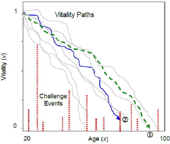
Figure 1: The two-process vitality model illustrated. Vitality declines stochastically from an initial value of 1. Intrinsic mortality results when adult vitality is exhausted, , and extrinsic mortality occurs when a random challenge exceeds the remaining vitality, .
2.2.1 Intrinsic mortality
The intrinsic mortality rate is governed by a gradual stochastic depletion of vitality over the life span according to equation (1). Without extrinsic killings, the first-passage time of vitality to the zero boundary is the inverse Gaussian distribution (Chhikara et al. 1989)
( )
⁄
√ (
( )
Pure intrinsic survival is
( ) ∫ ( ) (
√ ) (
) (
√ )
where is the cumulative normal distribution and the intrinsic mortality rate is
( ) ( ) ( )⁄ (2)
2.2.2 Extrinsic mortality
The extrinsic mortality rate depends on both the challenge occurrence rate and the challenge magnitude drawn from a cumulative distribution ( ), i.e., . Assume that the occurrence of challenges follows a Poisson process with rate ( ), such that a challenge at age does not depend on the previous history of challenges (Finkelstein 2007, 2008). Also, as in the SM theory, we assume challenges have a Maxwell-Boltzmann distribution such that most challenges are small and the probability of large challenges declines with magnitude (Strehler et al. 1960). Then the magnitude distribution is exponential and characterizes the mean challenge magnitude
( ) ⁄ (3)
Let ( ) denote the realization of the random vitality process , then the conditional extrinsic mortality rate is
( ∣∣ ( ) ) ( ) ( ) ( ) ( ( ( ))) ( ) ( ) ⁄ .
Integrating over vitality states, the population-level extrinsic rate is
( ) ∫ ( ∣∣ ) ( ) (4)
2.2.3 Total mortality – numerical model
Although the challenge process is assumed to be independent of the vitality process, the postulation that the extrinsic killing rate depends on the vitality level still evokes interactions between the intrinsic and extrinsic process. Therefore, the total mortality as the combination of the intrinsic and extrinsic deaths is not simply the sum of equations (2) and (4), but tends to carry some complexity due to the interactions of death processes. There is no analytical solution for the modified distribution of the Wiener process ( ) with the presence of extrinsic mortality and therefore for the total mortality rate. However, we can generate empirical mortality curves through microsimulation, which is a technique that numerically derives the average macro-level characteristics from repeated simulations at the individual level (Manton et al. 2009). In our case, we simulate thousands of individuals, each of which possesses its own vitality trajectory following the Wiener process with age (see Appendix for details). Independently, a Poisson process is generated to represent the random challenges with an exponentially distributed magnitude for each individual. The extrinsic death probability at age is calculated as the proportion of individuals for which the magnitude of a random challenge exceeds their vitality levels in the interval . Correspondingly, the intrinsic death probability in the interval is the proportion of individuals whose vitalities reach or pass through the zero-boundary. When either extrinsic or intrinsic death occurs, the individual’s vitality trajectory is stopped and the time to death recorded. The parameters , , and can be prescribed with any appropriate values, and in a more general sense all parameters can vary with age to yield nonhomogeneous processes in the simulation context. This approach generates age-specific mortality curves that fit empirical data. We refer to this as the numerical form of the model, or simply the “numerical model.”
Generating survival curves with the numerical model is computationally expensive and currently the approach is not amendable to estimation of parameters. Therefore, below we develop an analytical approximation to the vitality theory, i.e., the two-process vitality theory, amenable to parameter estimation. Then we correct the bias in parameters by fitting the modified model to survival curves generated by the numerical model.
2.2.4 Total mortality – modified model
To develop an approximate solution to the two-process vitality model, first assume that the extrinsic mortality depends on the mean vitality ̅( ) instead of the random variable
̃ ( ∣∣ ̅( ) ) ( ) ̅( ) ⁄ (5)
Next, note that to a first order the expected value of vitality according to equation (1) evolves linearly with age (Anderson et al. 2008) giving
̅( ) (6)
where is the initial vitality and in the normalized case is unity. Then the conditional extrinsic mortality defined by equation (4) becomes independent of the distribution of vitality and ( ) integrates to 1. Further, assuming the Poisson challenge process is homogeneous, i.e., ( ) , and then including equations (5) and (6) in (4), the modified extrinsic mortality rate is
̃ ( ) ( ) ⁄ (7)
where is the fraction of vitality loss per unit time and and are the frequency (occurrence rate) and the average magnitude of challenges. Equation (7) implies that at each age all individuals are subjected to the same average extrinsic killing force and hence the presence of extrinsic mortality does not change the vitality distribution resulting from the original Wiener process. With the sacrifice of randomness in extrinsic killing, the intrinsic and extrinsic mortality processes become independent of each other. Population heterogeneity is then only reflected in the intrinsic killing. Under these assumptions, the modified model for total mortality is the sum of equations (2) and (7) as
̃( ) ̃
⁄ ( ) ⁄
√ ( (
√ ) ⁄ (
√ ))
( ) ⁄
(8)
2.3 Fitting the model to data
In review, while the two-process theory cannot be expressed in a closed form, by assuming that the intrinsic and extrinsic processes work independently and that vitality in the extrinsic process is linear and non-stochastic, we are able to derive a close form of total mortality that can be fitted to data-yielding parameter estimates. The close form comes at a cost: the probability distribution describing intrinsic mortality does not account for the selective removal of lower vitality individuals by challenges, and the vitality used in the extrinsic mortality becomes negative at old age. Clearly, the modified form of the model cannot produce mortality patterns identical to patterns produced by the numerical model, but whether the modified model is sufficient depends on the task being addressed. In this paper we consider the adequacy of the modified model in three specific tasks: 1) comparing parameters across period years, 2) characterizing intrinsic and extrinsic mortality patterns with age, and 3) comparing the model to another model. In sections 2.3.1 – 2.3.3 we outline the methods for these assessments and report results in sections 3.1 – 3.3.
2.3.1 Parameter estimates
The first step in all tasks is developing unbiased estimates of model parameters. To estimate the bias-corrected parameters , , and for the modified model we first estimate biased parameters by fitting equation (8) to adult mortality curves (≥ 20 age) with a maximum-likelihood fitting routine (Salinger et al. 2003)3. We refer to these estimates as the biased parameters ( ̂ ̂ ̂ ̂). To develop bias corrections we simulate survival curves (see Appendix, Numerical simulation) using a range of “true parameters” centered over the biased parameters. We then fit the simulate mortality data with equation (8) to estimate biased parameters and develop regressions relating the true parameters to the biased parameters (see Appendix, Biases and corrections). Corrections to adjust biased parameters to real parameters are
̂ ̂ ̂ ̂ ̂ ̂ ̂̂ (9)
where the biased parameters are slightly low for and and slightly high for and .
3 R code for estimating parameters is available at http://CRAN.R-project.org/package=vitality. The package
2.3.2 Comparing age-dependence mortality patterns of models
To compare age-dependent patterns of intrinsic and extrinsic mortality generated by the modified model to those generated by the numerical model, we require numerical model parameter estimates that are functionally equivalent to the estimates for the modified model. First, we fit the modified model (equation 8) to period year mortality data and correct the parameters using equation (9). Second, we numerically simulate a mortality curve (see Appendix, Numerical simulation) based on these parameters. Third, we adjust the parameters within a small range, repeat the simulation, and continue the process until we find a set that yields a localized minimum root mean square error (RMSR) between the simulated mortality curve and the original data. In the simulations, trajectories of the two mortality components are generated from death numbers from intrinsic and extrinsic sources at each time interval.
2.3.3 Survival curve comparison
We compare the age-dependent patterns of mortality in the modified model with the three-parameter logistic model, which is the standard, low-parameter model for describing adult mortality (Thatcher 1999). The logistic model is ( )
where and are Gompertz parameters and is the Makeham term. The logistic model parameters are fit with the nonlinear least squares (nls) routine in R.
2.4 Application issues
Before moving on to the Results section, two important issues on the application of the model need to be considered.
2.4.1 Chronic vs. acute sources of mortality
challenges that increase the rate of vitality loss but do not result in immediate death. However, it is extremely difficult to distinguish the independent contributions of pure aging and pure environment changes to the loss of vitality (Carnes et al. 2006). Instead of seeking elusive distinctions between intrinsic and extrinsic causes of death, the model establishes a mathematically concise but admittedly imperfect partition in which both types of mortality are both age- and environment-related. A critical point is that extrinsic mortality is assumed to result from acute challenges that instantaneously drain the survival capacity of the individual, while intrinsic mortality is assumed to result from the chronic incremental losses of survival capacity to the point where it is simply exhausted. Of course, acute challenges that do not cause mortality can be manifested as chronic incremental losses of survival capacity, which thus links the two forms of mortality. We believe this approach provides insight into how historical changes in the environment and human health care shape mortality patterns, as well as offering a route to predict future mortality patterns.
2.4.2 Cohort data vs. Period data
more reflective of underlying processes than are parameters estimated from cohort data. We evaluate this prediction in the results section. In support of this hypothesis, a study comparing predictions of cancer mortality from period and cohort data found that the period data was a more accurate predictor of future rates (Brenner et al. 2008).
3. Results
We illustrate the ability of the model to fit period adult survival data using Swedish survival data from 1800 to 2007 downloaded from the Human Mortality Database, University of California, Berkeley (USA), and Max Planck Institute for Demographic Research (Germany). Available at www.mortality.org or www.humanmortality.de (data downloaded on 1/1/2010). All survival data are left-truncated at age 20 to exclude the child mortality processes.
3.1 Period survival curves
Model fits to Swedish female adult mortality data for the years 1820 and 2000 from the modified form of the model are illustrated in Figures 2A and 2C and fits with the numerical form of the model are illustrated in Figure 3. Note that the modified model curves are generated by fitting equation 8 with the maximum-likelihood routine, while the numerical model fits were obtained by searching the parameter space about parameters from Figure 2 after correcting for bias according to equation 9. Figure 2 parameters are the best global fit to the data while Figure 3 parameters represent the best fit to the data in the local parameter space.
The general patterns of the contributions of intrinsic and extrinsic mortality processes are the same with both forms of the models. Extrinsic mortality dominates the early portion of the curves and increases exponentially (linear in log space) in the modified model (Figures 2A, C) and asymptotes at old age in the numerical model (Figure 3). The extrinsic components for year 1820 have relatively shallow slopes, indicating that the extrinsic mortality rate has little age variation. In comparison, for year 2000 the extrinsic components rise steeply from low values in youth to high values at old age. In both model forms the intrinsic rates increase rapidly and equal or exceed the extrinsic rate at age 70 for the 1820 period and age 90 for the 2000 period. This difference in curves results because in 2000 is 30% smaller than in 1820. Finally, intrinsic mortality curves all approach a plateau at old age due to the Wiener-process nature of intrinsic mortality (Li et al. 2009; Weitz et al. 2001).
it continues to increase exponentially in the modified model. These differences result because, unlike in the numerical model, the modified model does not account for the removal of lower vitality individuals prior to old age. Thus extrinsic challenges act on a higher proportion of low-vitality individuals in the modified model than in the numerical model. In essence, with the numerical model, individuals surviving into old age have higher vitality than is predicted in the modified model.
3.2 Comparison of models
We compare the age-dependent patterns of mortality in the modified model with the three-parameter logistic model using adult Swedish female data for period years 1820 and 2000. Using the approach in a root-mean-squared-error (RMSE) comparison (Gage et al. 1993), fits to the modified model (Figure 2A and C) and the logistic model (Figure 2B and D) were similar for 1820, RMSE.vitality = 0.11 vs. RMSE.logistic = 0.12, but the logistic mortality model fits significantly worse for 2000 RMSE.vitality = 0.20 vs. RMSE.logistic = 0.31, p-value from the F test < 0.001(Gallant 1987).
Figure 2: Period adult mortality rate data (dots) of Swedish females for 1820 and 2000. (A) and (C): Model fits from the modified vitality model (equation 8). Modeled total mortality rate is depicted by red solid lines. Green dotted and blue dashed lines depict mortality compo-nents and . Model parameters are = 0.017, = 0.019, = 0.063, = 0.423 for year 1820 and = 0.013, = 0.011, = 0.148, = 0.139 for year 2000. (B) and (D): Logistic model fit depicted by red solid lines.
Mor
tal
it
y
rate
,
A B
Swedish Female (Mx, 1820)
total
e
iMor
tal
it
y
rate
,
Swedish Female (Mx, 2000)
total
i
eC D
Age,
x
Age,x
102102 1
104
1
Figure 3: Period adult mortality rate data (dots) of Swedish females for 1820 and 2000. Model fits from the numerical form of two-process vitality model. Modeled total mortality rate is depicted by red solid lines. Green dotted and blue dashed lines depict mortality components and . Model parameters are = 0.0174, = 0.015, = 0.062, = 0.426 for year 1820 and = 0.0138, = 0.007, = 0.118, = 0.143 for year 2000.
3.3 Historical patterns in survival
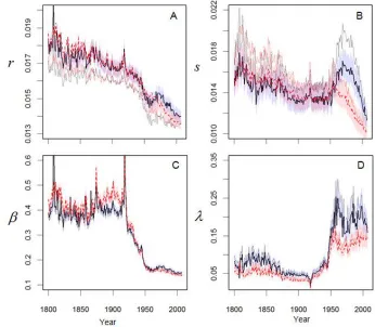
Here we demonstrate that the extraordinary improvements in human longevity (Riley 2001) across two centuries can be explained in terms of asynchronous across-year changes in the patterns of intrinsic and extrinsic process as characterized by the model parameters. Noting that is the rate of decline of vitality with age, and therefore a measure of the rate of aging, and the progressive decline in for both males and females (Figure 4A) quantifies the effects of improvements in living conditions across history. Studies suggest that improved nutrition and shelter associated with agrarian and industrial revolutions have reduced mortality rates (McKeown 1976; Riley 2001; Schofield 1991; Sundin et al. 2007), and thus are plausible mechanisms underlying the historical change in . By inference, the accelerated rate of decline of about 1940
Swedish Female (Mx)
M
or
tal
it
y
rate
,
A: 1820 B: 2000
total
e
i
Age,
x
1021
104
Age,
x
i
reflects a period of accelerated improvements in living conditions. Notably, after 1960
is higher in males than in females.
The intrinsic rate variability is a measure of heterogeneity in the rate of aging in the population. In the females, declines slowly over the 19th century, stabilizes in the first half of the 20th century, and, after a brief increase about 1950, declines in the late 20th century. The trend in males follows the female trend until 1950, at which time increases significantly through 1980 and then rapidly declines, suggesting a rapid increase and then decrease in the heterogeneity of aging in the male population (Figure 4B). This anomaly coincides with class-stratified differences in smoking rates in adult males over this 30-year span (Diderichsen 1990; Diderichsen et al. 1997). Additionally, the increase in between 1950 and about 1970 may reflect early effects of modernization, e.g., pollution and carcinogens (Crimmins 1981). Together and quantify the fundamental contributions of living conditions and health-related behaviors in shaping the pattern of intrinsic mortality in Sweden.
The extrinsic mortality, which is driven by environmental factors, exhibits three stages over the two-century record. In the first stage, up through 1920, the mean magnitude of environmental challenges (Figure 4C) is highly variable, plausibly resulting from variable environmental conditions associated with epidemics, fluctuations in food abundance, and climate. For example, spikes in in 1808 and 1918 respectively correspond with disease outbreaks associated with the Finnish war (Mielke et al. 1989) and the influenza pandemic (Sundin et al. 2007). The second stage, a decline in between 1920 and 1950, corresponds with a period in which many infectious diseases were controlled or eradicated (Omran 2005; Riley 2001). Improvements in health care that increased recovery rates from acute diseases (Finkelstein 2005) could also contribute to the decline. In the third stage, from 1950 onward, a low and stable reflects near elimination of high-magnitude challenges. Also noteworthy, is higher in 19th century females than males, which reflects preferential allocation of health resources to men at that time (Humphries 1991; Klasen 1998) as well as higher maternal mortality (Sundin et al. 2007).
environmental pollution and carcinogens, car accidents (Crimmins 1981), and exposure to disease related to public transportation, e.g., air and subway travel (Colizza et al. 2006).
The inverse pattern of and also alters the effect of extrinsic challenges with age. The 19th century high-magnitude challenges affect both young high-vitality individuals and old low-vitality individuals, resulting in a flatter extrinsic mortality curve (Figure 2A), while the 20th century low-magnitude challenges affect mostly old individuals with low vitality, resulting in a steeper curve (Figure 2C). Also note that across two centuries the challenge frequency is 20% less for females than males, which agrees with measured risk-taking differences between the sexes (Byrnes et al. 1999).
4. Comments
Demographic models of mortality have evolved, like species clades, from distinct conceptual foundations. The oldest clade, originating with Gompertz (1825), focuses on the mortality event itself as expressed through the hazard rate, and the issue is how the rate changes with age. The younger clade, beginning with Sacher (1956), takes a process point-of-view focusing on the processes leading up to death. The two clades have strengths and weaknesses. The hazard rate clade’s strength is through its simplicity and flexibility in characterizing age-dependent mortality, but it is weak in its difficulty in representing heterogeneity in survival capacity. The process point-of-view clade is weak in its representation of extrinsic events but strong in its stochastic representation survival capacity. In this paper we develop a framework that merges the fundamental processes of both clades into a single framework, one process describing extrinsic mortality in terms of external challenges to vitality and one process describing intrinsic mortality as the absorption of vitality into a zero boundary.
Vitality, the abstract stochastic measure of survival capacity, is the shared currency for both processes, which leads to conceptual and mathematical challenges in formulating a tractable low-parameter model. Challenges preferentially kill low vitality individuals and therefore the vitality distribution determining intrinsic mortality is affected by extrinsic processes. Additionally, challenges not resulting in death affect the rate of loss of vitality, further affecting intrinsic processes. A focus of our paper has been to decouple this interaction while retaining important properties of the framework. We proceeded in three stages. We first developed the conceptual framework, which has no closed-form mortality equation but which is amenable to numerical simulation. Next, we derived a close-form model that decouples the intrinsic and extrinsic processes. Third, we compared the close-form model to the numerical simulations to correct for the biases resulting from decoupling the processes. The final modified model contains only four parameters and is suitable for analysis of empirical data in estimation algorithms. Furthermore, mortality rate deviations from classical exponential increases are readily explained by simple biologically realistic intrinsic and extrinsic processes.
The vitality framework has considerable flexibility, but to obtain a tractable model the framework must be simplified, resulting in conceptual and parameter estimation issues. For example, estimates of the extrinsic mortality parameters are highly sensitive to deviations of challenges from a Maxwell-Boltzmann distribution. This is particularly critical if the nature of environmental challenges change quickly, such as might be expected with climate change. Other issues need further consideration. Clearly, nonlethal injuries and disease affect vitality, and therefore longevity, but the model ignores such interactions. Also, the framework currently is not applicable to early life development where vitality is expected to increase instead of decline. Notwithstanding these limitations, the simplicity in characterizing intrinsic and extrinsic mortality processes by four parameters offers considerable insight into what shapes patterns of mortality. We suggest that models that do not explicitly represent both intrinsic and extrinsic processes are inadequate to understand historical mortality patterns and predict future patterns. Thus, in summary, we believe that a vitality-based theory offers a rigorous and tractable framework which links these processes.
5. Acknowledgements
References
Aalen, O.O. and Gjessing, H.K. (2001). Understanding the shape of the hazard rate: A process point of view. Statistical Science 16(1): 1-22. doi:10.1214/ss/998 929472.
Anderson, J.J. (1992). A vitality-based stochastic model for organism survival. In: DeAngelis, D.L. and Gross, L.J. (eds.). Individual-based models and approaches in ecology: Populations, communities and ecosystems. New York: Chapman & Hall: 256–277.
Anderson, J.J. (2000). A vitality-based model relating stressors and environmental properties to organism survival. Ecological Monographs 70(3): 445-470.
doi:10.1890/0012-9615(2000)070[0445:AVBMRS]2.0.CO;2.
Anderson, J.J., Gildea, M.C., Williams, D.W., and Li, T. (2008). Linking growth, survival, and heterogeneity through vitality. The American Naturalist 171(1): E20-E43. doi:10.1086/524199.
Bongaarts, J. (2006). How long will we live? Population and Development Review
32(4): 605-628. doi:10.1111/j.1728-4457.2006.00144.x.
Brenner, H. and Hakulinen, T. (2008). Period versus cohort modeling of up-to-date cancer survival. International Journal of Cancer 122(4): 898-904. doi:10.1002/ ijc.23087.
Byrnes, J.P., Miller, D.C. and Schafer, W.D. (1999). Gender differences in risk taking: A meta-analysis. Psychological Bulletin 125(3): 367-383. doi:10.1037/0033-2909.125.3.367.
Carnes, B.A., Holden, L.R., Olshansky, S.J., Witten, M.T., and Siegel, J.S. (2006). Mortality partitions and their relevance to research on senescence.
Biogerontology 7(4): 183-198. doi:10.1007/s10522-006-9020-3.
Carnes, B.A. and Olshansky, S.J. (1997). A biologically motivated partitioning of mortality. Experimental Gerontology 32(6): 615-631.
doi:10.1016/S0531-5565(97)00056-9.
Carnes, B.A., Olshansky, S.J., and Grahn, D. (1996). Continuing the search for a law of mortality. Population and Development Review 22(2): 231-264. doi:10.2172/ 206929.
Colizza, V., Barrat, A., Barthélemy, M., and Vespignani, A. (2006). The role of the airline transportation network in the prediction and predictability of global epidemics. Proceedings of the National Academy of Sciences of the United States of America 103(7): 2015-2020. doi:10.1073/pnas.0510525103.
Crimmins, E.M. (1981). The changing pattern of American mortality decline, 1940-77, and its implications for the future. Population and Development Review 7(2): 229-254. doi:10.2307/1972622.
Diderichsen, F. (1990). Health and social inequities in Sweden. Social Science & Medicine 31(3): 359-367. doi:10.1016/0277-9536(90)90283-X.
Diderichsen, F. and Hallqvist, J. (1997). Trends in occupational mortality among middle-aged men in Sweden 1961-1990. International Journal of Epidemiology
26(4): 782-787. doi:10.1093/ije/26.4.782.
Finkelstein, M.S. (2007). Aging: Damage accumulation versus increasing mortality rate. Mathematical Biosciences 207(1): 104-112. doi:10.1016/j.mbs.2006. 09.007.
Finkelstein, M.S. (2008). Failure rate modelling for reliability and risk. New York: Springer Verlag.
Finkelstein, M.S. (2005). Lifesaving explains mortality decline with time.
Mathematical Biosciences 196(2): 187-197. doi:10.1016/j.mbs.2005.04.004.
Gage, T.B. and Mode, C.J. (1993). Some laws of mortality: How well do they fit?
Human Biology 65(3): 445-461.
Gallant, A.R. (1987). Nonlinear statistical models. NJ, USA: John Wiley & Sons, Inc., Hoboken. doi:10.1002/9780470316719.
Golubev, A. (2009). How could the Gompertz-Makeham law evolve. Journal of Theoretical Biology 258(1): 1-17. doi:10.1016/j.jtbi.2009.01.009.
Gompertz, B. (1825). On the nature of the function expressive of the law of human mortality, and on a new mode of determining the value of life contingencies.
Philosophical Transaction of the Royal Society of London 115: 513-583. doi:10.1098/rstl.1825.0026.
Heligman, L. and Pollard, J.H. (1980). The age pattern of mortality. Journal of the Institute of Actuaries 107(1): 49-80. doi:10.1017/S0020268100040257.
Humphries, J. (1991). "Bread and a pennyworth of treacle": Excess female mortality in England in the 1840s. Cambridge Journal of Economics 15(4): 451-473.
Klasen, S. (1998). Marriage, bargaining, and intrahousehold resource allocation: Excess female mortality among adults during early German development, 1740-1860.
Journal of Economic History 58(2): 432-467. doi:10.1017/S00220507
0002057X.
Krementsova, A.V. and Gorbunova, N.V. (2010). The impact of environment on lifespan distribution dynamics. Automation and Remote Control 71(8): 1617-1628. doi:10.1134/S0005117910080114.
Li, T. and Anderson, J.J. (2009). The vitality model: A way to understand population survival and demographic heterogeneity. Theoretical Population Biology 76(2): 118-131. doi:10.1016/j.tpb.2009.05.004.
Makeham, W.M. (1860). On the law of mortality and the construction of annuity tables.
Journal of the Institute of Actuaries 8: 301-310.
Manton, K.G., Akushevich, I. and Kravchenko, J. (2009). Cancer mortality and morbidity patterns in the US population: An interdisciplinary approach. New York: Springer Verlag. doi:10.1007/978-0-387-78193-8.
McKeown, T. (1976). The modern rise of population. London: Edward Arnold.
Mielke, J.H. and Pitkänen, K.J. (1989). War demography: The impact of the 1808-09 war on the civilian population of Åland, Finland. European Journal of Population / Revue Européenne de Démographie 5(4): 373-398.
Oeppen, J. and Vaupel, J.W. (2002). Broken limits to life expectancy. Science
296(5570): 1029-1031. doi:10.1126/science.1069675.
Olshansky, S.J. (2010). The law of mortality revisited: Interspecies comparisons of mortality. Journal of Comparative Pathology 142(Supplement 1): S4-S9. doi:10.1016/j.jcpa.2009.10.016.
Olshansky, S.J., Carnes, B.A., and Cassel, C. (1990). In search of Methuselah: Estimating the upper limits to human longevity. Science 250(4981): 634-640. doi:10.1126/science.2237414.
Omran, A.R. (2005). The epidemiologic transition: A theory of the epidemiology of population change. Milbank Quarterly 83(4): 731-757.
doi:10.1111/j.1468-0009.2005.00398.x.
Passos, J.F. and von Zglinicki, T. (2005). Mitochondria, telomeres and cell senescence.
Riggs, J.E. (1990). Longitudinal Gompertzian analysis of adult mortality in the U.S., 1900-1986. Mechanisms of Ageing and Development 54(3): 235-247.
doi:10.1016/0047-6374(90)90053-I.
Riggs, J.E. and Millecchia, R.J. (1992). Using the Gompertz-Strehler model of aging and mortality to explain mortality trends in industrialized countries. Mechanisms of Ageing and Development 65(2-3): 217-228.
doi:10.1016/0047-6374(92)90037-E.
Riley, J.C. (2001). Rising life expectancy: A global history. New York: Cambridge University Press.
Sacher, G.A. (1956). On the statistical nature of mortality, with especial reference to chronic radiation mortality. Radiology 67(2): 250-258.
Salinger, D.H., Anderson, J.J., and Hamel, O.S. (2003). A parameter estimation routine for the vitality-based survival model. Ecological Modelling 166(3): 287-294.
doi:10.1016/S0304-3800(03)00162-5.
Schofield, R., Reher, D.S., and Bideau, A. (1991). The decline of mortality in Europe.
Oxford University Press.
Siler, W. (1979). A competing-risk model for animal mortality. Ecology 60(4): 750-757. doi:10.2307/1936612.
Steinsaltz, D. and Evans, S.N. (2004). Markov mortality models: Implications of quasistationarity and varying initial distributions. Theoretical Population Biology 65(4): 319-337. doi:10.1016/j.tpb.2003.10.007.
Strehler, B.L. and Mildvan, A.S. (1960). General theory of mortality and aging. Science
132(3418): 14-21. doi:10.1126/science.132.3418.14.
Sundin, J. and Willner, S. (2007). Social change and health in Sweden: 250 years of politics and practice. Stockholm: Swedish National Institute of Public Health.
Thatcher, A. R. (1999). The long-term pattern of adult mortality and the highest attained age. Journal of the Royal Statistical Society: Series A (Statistics in Society) 162(1): 5-43.
Vaupel, J.W. (2010). Biodemography of human ageing. Nature 464(7288): 536-542. doi:10.1038/nature08984.
Vaupel, J.W., Manton, K.G., and Stallard, E. (1979). The impact of heterogeneity in individual frailty on the dynamics of mortality. Demography 16(3): 439-454.
Weitz, J.S. and Fraser, H.B. (2001). Explaining mortality rate plateaus. Proceedings of the National Academy of Sciences of the United States of America 98(26): 15383-6. doi:10.1073/pnas.261228098.
Yashin, A.I., Begun, A.S., Boiko, S.I., Ukraintseva, S.V., and Oeppen, J. (2001a). The new trends in survival improvement require a revision of traditional gerontological concepts. Experimental Gerontology 37(1): 157-167.
doi:10.1016/S0531-5565(01)00154-1.
Yashin, A.I., Begun, A.S., Boiko, S.I., Ukraintseva, S.V. and Oeppen, J. (2001b). Recent trends in survival improvement set up new problems for biodemographic research. Gerontologist 41: 85.
Yashin, A.I., Begun, A.S., Boiko, S.I., Ukraintseva, S.V., and Oeppen, J. (2002). New age patterns of survival improvement in Sweden: Do they characterize changes in individual aging? Mechanisms of Ageing and Development 123(6): 637-647.
doi:10.1016/S0047-6374(01)00410-9.
Yashin, A.I., Iachine, I.A., and Begun, A.S. (2000). Mortality modeling: A review.
Mathematical Population Studies 8(4): 305-332. doi:10.1080/08898480009 525489.
Zheng, H., Yang, Y., and Land, K.C. (2011). Heterogeneity in the Strehler-Mildvan general theory of mortality and aging. Demography 48(1): 267-290.
Appendix
Evaluating model parameter bias: We conducted microsimulation to evaluate the modified model, which expressed by equation (8) assumes that the effect of the extrinsic challenge can be represented by an approximation of the mean vitality at age . Survival curves were generated according to a vitality process defined by equation (1) with pre-assigned parameters in which extrinsic process kills individuals according to their actual vitality level and otherwise mortality occurs at the zero boundary. The modified model was then fitted with the numerically generated curves to obtain estimated parameters, which were then compared to the true parameter values for assessing the bias inherent in the modified model.
Numerical simulation: Survival curves were simulated from the vitality process defined by equation (1). Each population member was assumed to have a vitality of 1 at age 0. The vitality for each individual was calculated for a single age step as
(A1)
where is an increment of the Weiner process simulated by a random number from a unit normal distribution N[0,1]. Note that this generation uses a simplified random walk with drift to approximate the continuous Wiener process. From (A1), 10,000 vitality trajectories were generated to represent a population. At each age , deaths from intrinsic and extrinsic process were recorded. Mortality from extrinsic challenges was defined by a probability distribution where the probability of dying from the extrinsic process in age interval ( ) equals
( ∫ ⁄
) ( ( ⁄ ⁄ ))
which mimics the random Poisson challenge process with an exponentially distributed magnitude. An intrinsic mortality event was defined when an individual’s vitality trajectory dropped below zero. In both cases the vitality trajectory was excluded from further calculations. Thus survival curves were calculated from the fraction of vitality trajectories remaining at each age.
Biases and corrections: We aimed to correct the bias of the model parameters
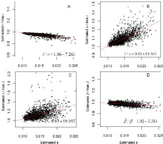
slightly underestimated, and and are overestimated by less than 40% of their true values. To investigate the bias of parameters estimated from human mortality data we conducted simulations based on parameters obtained from period mortality data of adult (age 20) Swedish females (1800-2007) according to equation (8). For each period year a set of parameters ( ̂ ̂ ̂ ̂) was estimated from the Swedish mortality curve using the two-process model-fitting algorithm in the vitality package in CRAN (http://CRAN.R-project.org/package=vitality). Thus there were 208 baseline parameter sets. Ten additional parameter sets were randomly picked for each of the four parameters, allowing , and to vary separately within a range from 95% to 100%, 60 to 100%, 70% to 100%, and 95% to 105% of their baseline values, which gave in total 2080 = 208×10 “true” parameter sets. We generated 2080 survival curves according to the process, estimated 2080 parameter sets, and compared them to the “true” sets, which were used to estimate the bias corrections for the parameters.
Figure A1: Numerical simulations depicting the effect of model assumptions on biasing parameter estimates depicted as ratios of estimated
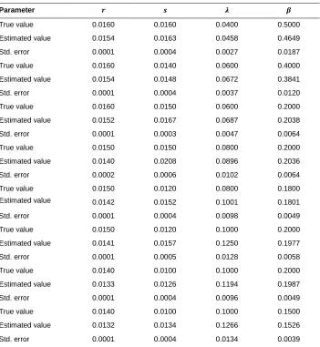
Table A1: Results from the analysis of parameter bias where parameters are chosen close to the values estimated from the morality data of Swedish females.
Parameter
True value 0.0160 0.0160 0.0400 0.5000
Estimated value 0.0154 0.0163 0.0458 0.4649
Std. error 0.0001 0.0004 0.0027 0.0187
True value 0.0160 0.0140 0.0600 0.4000
Estimated value 0.0154 0.0148 0.0672 0.3841
Std. error 0.0001 0.0004 0.0037 0.0120
True value 0.0160 0.0150 0.0600 0.2000
Estimated value 0.0152 0.0167 0.0687 0.2038
Std. error 0.0001 0.0003 0.0047 0.0064
True value 0.0150 0.0150 0.0800 0.2000
Estimated value 0.0140 0.0208 0.0896 0.2036
Std. error 0.0002 0.0006 0.0102 0.0064
True value 0.0150 0.0120 0.0800 0.1800
Estimated value 0.0142 0.0152 0.1001 0.1801
Std. error 0.0001 0.0004 0.0098 0.0049
True value 0.0150 0.0120 0.1000 0.2000
Estimated value 0.0141 0.0157 0.1250 0.1977
Std. error 0.0001 0.0005 0.0128 0.0058
True value 0.0140 0.0100 0.1000 0.2000
Estimated value 0.0133 0.0126 0.1194 0.1987
Std. error 0.0001 0.0004 0.0096 0.0049
True value 0.0140 0.0100 0.1000 0.1500
Estimated value 0.0132 0.0134 0.1266 0.1526
Challenge distribution effect on challenge frequency: To evaluate if the increase in challenge frequency after 1950 (Figure 4D) could be the result of the distribution function of challenge magnitude ( ̅( )) deviating from the assumed exponential pattern, we conducted simulations. We specified two types of challenges. Type 1 challenges had higher average magnitude and lower frequency , as might be expected with extreme, but rare, disease outbreaks and natural disasters. Type 2 challenges had lower average magnitude but higher frequency , as might be expected with physical injuries and common diseases. The challenge magnitudes for both types followed exponential distributions. Survival curves were generated following the method described in the survival curve generation algorithm of equation (A1). Both types of challenges were applied to the population. Parameters = 0.014, = 0.01, = 0.15, = 0.5 and = 0.12 were fixed and was varied from 0 to 0.05. The simulation results, summarized in Figure A2, depict the ratios of the estimated parameters to the true or expected values in the simulations plotted against . The expected challenge frequency is the sum of the two frequencies,
(A2)
and the expected challenge magnitude is the weighted magnitude from the two sources
(A3)
As suggested by Figure A2, the decrease in frequency for the high magnitude challenges does not significantly influence and . However, the ratio of declines slightly and the ratio of fluctuates as the frequency of the higher magnitude challenge is reduced. Thus the intrinsic parameters are relatively insensitive to variations in the nature of challenges. In contrast, the challenge parameters are sensitive to the mixture of challenges. With a relatively large proportion of Type 1 challenges, the estimated is biased to , but when the frequency of Type 1 challenges is reduced to a threshold, i.e., , in the simulation, the estimated quickly approaches its expected value . The estimated is also affected. When Type 1 challenges dominate, the average challenge magnitude is overestimated. Also, when Type 2 challenges dominate, the estimated magnitude approaches that predicted by equation (A3). Thus, the model assumption that all challenges can be represented by a single distribution function results in biases when the challenges are comprised of different distributions of frequencies and magnitudes. Therefore, the challenge parameters we obtained from the model may best reflect the characteristics of high magnitude challenges.