49
The Karkheh River Streamflow Forecast based on the
Modelling of Time Series
Karim Hamidi Machekposhti 1, Hossein Sedghi 1*, Abdolrasoul Telvari 2, Hossein Babazadeh 1 1 Department of Water Sciences and Engineering, Science and Research Branch, Islamic Azad University, Tehran,
Iran
1* Department of Water Sciences and Engineering, Science and Research Branch, Islamic Azad University, Tehran, Iran ([email protected])
2 Department of Civil Engineering, Ahvaz Branch, Islamic Azad University, Ahvaz, Iran
1 Department of Water Sciences and Engineering, Science and Research Branch, Islamic Azad University, Tehran, Iran
(Date of received: 30/01/2018, Date of accepted: 18/04/2019)
ABSTRACT
Autoregressive integrated moving average (ARIMA) models are appropriate for the annual streamflows (annual peak and maximum and also mean discharges) of the Karkheh River at Jelogir Majin station of Karkheh river basin in Khuzestan province in western Iran, through the Box- Jenkins time series modelling approach. In this research among the suggested models interpreted from ACF and PACF, ARIMA(4,1,1) for all annual streamflows satisfied all tests and showed the best performance. The model forecasted streamflow for ten leading years showed the ability of the model to forecast statistical properties of the streamflow in short time in future. The SAS and SPSS softwares were used to implement of the models.
Keywords:
50
technology has broadened to encompass the problems of both surface water and groundwater systems. With such a broad domain, statistics has emerged as a powerful tool for analyzing hydrologic time series. The Box-Jenkins ARIMA model is the most commonly time series model in hydrologic time series modelling [1]. The ARIMA model has two general forms: ARIMA(p, d, q) and multiplicative ARIMA(p, d, q)×(P,D,Q) in which p and q are non-seasonal autoregressive and moving average, P and Q are seasonal autoregressive and moving average parameters, respectively. The other two parameters, d and D, are required differencing used to make the series stationary. Several researches have conducted about streamflows time series modelling in the world [2, 3, 4, 5, 6, 7, and 8].
2. Study Area
51
Figure 1. The Study area location.
3. Material and Methods
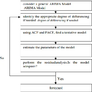
The Box and Jenkins modelling approach has three steps. Model identification is the first step. The second step is to estimate parameters and diagnostic checking, and the last step is to apply goodness of fit test. In this step, the model that seems to represent the behavior of the series is searched through autocorrelation and partial autocorrelation functions (ACF and PACF) for further investigation and parameter estimation [9].
After identifying models, we need to obtain efficient estimates of the parameters. Several methods are available for estimating parameters including Maximum Likelihood (ML), Conditional Least Squares (CLS) and Unconditional Least Squares (ULS). Among these methods, maximum likelihood and conditional least squares seems to be the best [1, 9]. The parameters should be statistically significant at α= p% and satisfy two conditions, namely stationary and invert ability for autoregressive and moving average models, respectively. The third step, Goodness of fit tests, verifies the validity of the model using some tools. The residuals of the model are usually considered to be time independent and normally distributed over time. The most common tests applied to test time, independence and normality, are the Portmanteau lack of fit test, the nonparametric Kolmogrov–Smirnov and Anderson–Darling tests [10]. The Statistical Analysis System (SAS) and Statistical Package for the Social Science (SPSS) softwares were used to for determinate of the best model for this series. The basic methodology of ARIMA development (Box and Jenkins modelling approach) is shown in Figure 2:
Figure 2. ARIMA model development.
52
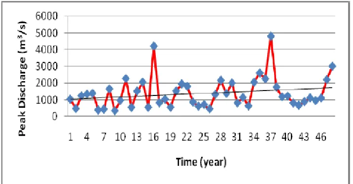
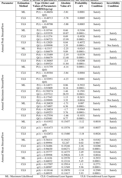
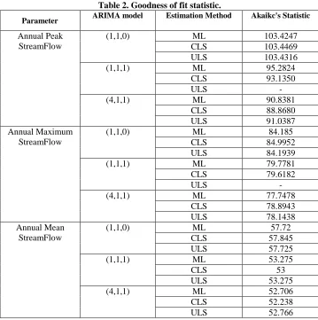
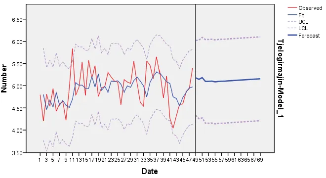
there is increase trend for studied series. In this study, the Ln of natural series is not stationary and then has first differencing of Ln natural data to achieving stationary series (d=1. Therefore, the optimum level of differencing for the series was one and the d value used in the ARIMA model would be one (d=1). We try to fit an ARIMA model to the annual streamflow of the Karkheh River. We use annual streamflow such as peak and maximum and also mean discharge time series of this river in Jelogir Majin hydrometric station the period 1958-2005. Based on the ACF and PACF of the logarithmic series, three models are examined for further consideration. The first model is ARIMA(1,1,0), the second is ARIMA(1,1,1) and the third is ARIMA(4,1,1). All three models were suitable for modelling (Table 1). According to Akaike index (Table 2) the best model was ARIMA (4,1,1). The results of time independent and normal test of residuals show the adequacy of the three model estimated by CLS and ML methods. Therefore, the model ARIMA (4,1,1) for peak and mean discharge whose parameters are estimated by CLS method is the best model and the model ARIMA(4,1,1) for maximum discharge whose parameters are estimated by ML method is the best model. Figures 6-8 shows the model prediction and observed annual streamflow of the Karkhe River which match well together. The above selected model was then used for forecasting streamflow from 2006 to 2015 (Table 3). Comparing the observed and model forecasted streamflow indicates the same yearly variation for all series. This may imply the capability of the ARIMA model in forecasting.
53
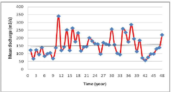
Figure 4. Original annual maximum streamflow (Discharge) time series.
54 An n u al Peak Stre am Flo w Q(0)
CLS P(1) = -0.48713
Q(0)
-3.78 0.0005 Satisfy
ULS P(1) = -0.49708
Q(0)
-3.88 0.0003 Satisfy
ML P(1) = 0.10744
Q(1) = 0.93539
0.66 10.87 0.5104 0.0001< Satisfy Satisfy
CLS P(1) = 0.11274
Q(1) = 0.96723
0.69 15.99 0.4926 0.0001< Satisfy Satisfy
ULS P(1) = 0.12820
Q(1) = 0.99998
0.84 3.35 0.4072 0.0001< Satisfy Not Satisfy
ML P(4) = -0.3317
Q(1) = 0.86679
-2.25 9.89 0.0243 0.0001< Satisfy Satisfy
CLS P(4) = -0.33489
Q(1) = 0.86679
-2.19 13.48 0.0339 0.0001< Satisfy Satisfy
ULS P(4) = -0.36065
Q(1) = 0.89524
-2.4 11.84 0.0208 0.0001< Satisfy Satisfy An n u al Ma x im u m Stre am Flo w
ML P(1) = -0.51759
Q(0)
-4.14 0.0001< Satisfy
CLS P(1) = -0.49304
Q(0)
-3.84 0.0004 Satisfy
ULS P(1) = -0.52951
Q(0)
-4.23 0.0001 Satisfy
ML P(1) = 0.14873
Q(1) = 0.92809
0.86 8.16 0.3922 0.0001< Satisfy Satisfy
CLS P(1) = 0.230274
Q(1) = 0.97512
1.46 28.55 0.1501 0.0001< Satisfy Satisfy
ULS P(1) = 0.17543
Q(1) = 0.99999
1.13 3.35 0.2631 0.0016 Satisfy Not Satisfy
ML P(4) = -0.26820
Q(1) = 0.74897
-1.71 6.36 0.087 0.0001< Satisfy Satisfy
CLS P(4) = -0.26824
Q(1) = 0.69253
-1.7 5.76 0.0964 0.0001< Satisfy Satisfy
ULS P(4) = -0.27556
Q(1) = 0.85681
-1.66 8.77 0.1031 0.0001< Satisfy Satisfy An n u al Me an Stre am Flo w
ML p(1) = -0.41932
q(0)
0.13457 -3.12 0.0018 Satisfy
CLS p(1) = -0.41473
q(0)
0.13576 -3.05 0.0037 Satisfy
ULS p(1) = -0.42872
q(0)
0.13480 -3.18 0.0026 Satisfy
ML p(1) = 0.36414
q(1) = 0.99994
0.15423 52.247 2.36 0.02 0.0182 0.9847 Satisfy
CLS p(1) = 0.34486
q(1) = 0.96630
0.15246 0.04271 2.26 22.62 0.0286 0.0001< Satisfy
ULS p(1) = 0.35777
q(1) = 0.99998
0.14375 0.29826 2.49 3.35 0.0166 0.0016 Satisfy
ML p(4) = -0.1636
q(1) = 0.66032
0.15570 0.12124 -1.5 5.45 0.2933 0.0001< Satisfy
CLS p(4) = -0.17507
q(1) = 0.68987
0.15914 0.11569 -1.1 5.96 0.2771 0.0001< Satisfy
ULS p(4) = -0.18146
q(1) = 0.68935
0.15870 0.11617 -1.14 5.93 0.2589 0.0001< Satisfy
55
Table 2. Goodness of fit statistic.
Parameter ARIMA model Estimation Method Akaikc's Statistic
Annual Peak StreamFlow
(1,1,0) ML 103.4247
CLS 103.4469 ULS 103.4316
(1,1,1) ML 95.2824
CLS 93.1350
ULS
-(4,1,1) ML 90.8381
CLS 88.8680
ULS 91.0387
Annual Maximum StreamFlow
(1,1,0) ML 84.185
CLS 84.9952
ULS 84.1939
(1,1,1) ML 79.7781
CLS 79.6182
ULS
-(4,1,1) ML 77.7478
CLS 78.8943
ULS 78.1438
Annual Mean StreamFlow
(1,1,0) ML 57.72
CLS 57.845
ULS 57.725
(1,1,1) ML 53.275
CLS 53
ULS 53.275
(4,1,1) ML 52.706
CLS 52.238
ULS 52.766
Table 3. Forecasts from period 2006-7 to 2015-16.
Period
Forecast
Annual Peak StreamFlow
Annual Maximum StreamFlow
Annual Mean StreamFlow
2006-7 1451.13 1234.6 138.9
2007-8 1384.65 1176.4 132.5
2008-9 1091.6 962.1 130.9
2009-10 983.980 919.2 120.7
2010-11 1256.52 1091.7 130.8
2011-12 1276.4 1106 131.9
2012-13 1382.16 1167.2 132.2
2013-14 1431.11 1181.7 134
2014-15 1318.57 1128.3 132.2
56
Figure 6. Observed and model prediction of peak streamflow of Karkheh river.
Figure 7. Observed and model prediction of maximum streamflow of Karkheh river.
57 5. Conclusions and Discussions
In this research, we attempted to forecast Karkheh river streamflow in Jelogir Majin station (upstream of Karkheh dam reservoir) in Karkheh river basin at Iran using time series modelling (ARIMA models). The ARIMA model has a better performance than other ARMA stochastic model because it makes time series stationary, in forecasting. The model ARIMA (4,1,1) was fitted to annual streamflow in this river. Accepted model in this station give us ten years predicted along with their 95% confidence interval that can help decision makers to establish strategies, priorities and proper use of water resources in this river at Iran. The ARIMA models are suitable for short term forecasting because the ARMA family models can model short term persistence very well. These models are a finite memory model, thus it does not fare well in long term forecasting. The significant ACF and PACF functions with high order can be caused by factors such as area good vegetation and water from snowmelt. The good vegetation of the region and the forest causes water retention in the soil surface layer and delay in the rise in surface runoff. As well as vegetation reduces the power and erodibility destroyed by a severe storm (intense rain events happening across the region) and runoff from the storm drainage system seems to cause significant delays.
6. References
[1]- Box, G. E. P. and Jenkins, G. M., 1976, Time Series Analysis, Forecasting and Control, Holden Day. San Francisco. California.
[2]- Shakeel, A. M., Idrees, A. M., Naeem, H. M., and Sarwar, B. M., 1993, Time Series Modelling
of Annual Maximum Flow of River Indus at Sukkur. Pakistan, Journal of Agricultural
Sciences, 30(1), 36-38.
[3]- Srikanthan, R., McMohan,T. A. and Irish, J. L., 1983, Time series analysis of annualflows
of Australian streams, Journal of Hydrology, 1, 12-21.
[4]- Stojković, M., Prohaska, S. and Plavšić, J., 2015, Stochastic Structure of Annual discharges
of large European Rivers, Journal of Hydrology and Hydromechanics, 63(1), 63–70.
[5]- Nigam, R., Nigam, S., and Mittal, S. K., 2014, The river runoff forecast based on the
modeling of time series, Russian Meteorology and Hydrology, 39(11), 750-761.
[6]- Tian, P., Zhao, G. J., Li, J., and Tian, K., 2011, Extreme Value Analysis of Stream flow
Time Series in Poyang Lake Basin, China, Water Science and Engineering, 4(2), 121-132.
[7]- Shahjahan, M. M., and Chowdhury, J. U., 2013, Generation of 10-Day flow of the
Brahmaputra River using a time series model, Hydrology Research, 44(6), 1071-1083.
[8]- Hamidi machekposhti, K., Sedghi, H., Telvari, A., and Babazadeh, H., 2017, Forecasting by
Stochastic Models to Inflow of Karkheh Dam at Iran, Civil Engineering Journal, 3(5): 340-350.
[9]- McLeod, A. E., Hipel, K. W. and Lennox, W. C., 1977, Advances in Box- Jenkins modeling:
2- Applications,Water Resources Research, 13(3), 577-586.
[10]- Modarres, R., and Eslamian, S. S., 2006, Streamflows time series modeling of
Zayandehrud River, Iranian Journal of Science & Technology, Transaction B, Engineering,