0 INTRODUCTION
Cavitation is the formation and then immediate implosion of cavities in a liquid that are the consequence of forces acting upon the liquid. It usually occurs when a liquid is subjected to rapid changes of pressure or velocity. Cavitation can cause different undesirable effects, such as performance loss, damage by pitting and erosion, structure vibrations and noise generation in the machinery.
Cavitation can take different forms, depending on hydrodynamic conditions. Stable cavities, defined as sheet cavitation, may develop in the low pressure regions attached on solid walls. If sheet cavity increases over the critical size, periodic fluctuations of cavity appear. These oscillations are accompanied with adverse pressure gradients and downstream shedding of clouds. The cavitation cloud shedding in the wake of cylindrical bluff body is the subject of present study.
Many numerical and experimental studies on cavitating flows have been performed. The numerical studies, performed nowdays mainly focus either on mathematical and physical model development [1], its optimization [2] or on cavitation erosion prediction [3]. The experimental studies have longer history. Pioneer work for the case of cavitation flow visualization around a hydrofoil was carried out by Wade and Acosta [4] in 1966. The major aim of study was to measure lift and drag coefficients of the
hydrofoil with and without the presence of cavity oscillations.
Several studies were performed where frequency of cavitation clouds shedding was analysed. Among them are Kjeldsen et al. [5] who classified the types and length of cavitation by a combination of angle of attack and cavitation coefficient , and compared the range of periodical shedding of the cloud cavitation to the Strouhal number. The experiments performed by George et al. [6] revealed that oscillations of cavitation clouds possess similar range of Strouhal numbers. Cavitation clouds have complex structure and behavior. Measurements performed by Kubota et al. [7] showed that the cloud cavity consisted of a large-scale vortex and cluster of small vapor bubbles located in the center of the vortex. Such complexity of cavitation clouds is reflected in periodic nature and variability of pressure oscillations. Pressure oscillations were measured using piezo-electric transmitters and their classification into local and global pulses was performed by Reisman and Brennen [8].
The development of modern visualization techniques resulted in detailed shedding phenomena and frequency content investigation performed on a case of spherical bluff body by Brandner et al. [9].
Strongly connected to this paper are studies about simultaneous pressure measurements and visualization of cavitation cloud structure using high speed imaging. Reisman et al. [10] studied shock waves in cloud cavitation using high speed visualization and
The Experimental Analysis of Cavitating Structure Fluctuations
and Pressure Pulsations in the Cavitation Station
Biluš, I. – Bombek, G. – Hočevar, M. – Širok, B. – Cenčič, T. – Petkovšek, M.Ignacijo Biluš1,* – Gorazd Bombek1 – Marko Hočevar2 – Branko Širok2 – Tine Cenčič2 – Martin Petkovšek2
1 University of Maribor, Faculty of Mechanical Engineering, Slovenia 2 University of Ljubljana, Faculty of Mechanical Engineering, Slovenia
The experimental analysis of unsteady cavitating flow has been performed to compare the static pressure dynamics and cavitation cloud structure dynamics. The analysis of the unsteady cavitation flow field was performed in the wake of bluff body in the laboratory cavitation station. The pressure oscillations were measured downstream of the bluff body with a recessed installation of the pressure sensor. The cavitation cloud structure dynamics was visualized using high speed camera. Pressure and image acquisition was performed simultaneously. The results of both measurements were analyzed in low frequency and high frequency intervals. The low frequency analysis of both pressure and cloud structure oscillations was performed in the interval from 0 to 1000 Hz. The high frequency analysis of the pressure fluctuations was performed with band pass filtering from 300 to 400 kHz and amplitude demodulation. Comparison of the static pressure and cavitation cloud structures fluctuations caused by cavitation cloud shedding in the wake of bluff body showed similarity between both signals. Two distinct frequencies of flow oscillations were recognized and the influence of cavitation number on the strength of pressure and cloud structure oscillations was quantified. The amplitude demodulation method was used to show and discuss the connection between the low and high frequency pressure oscillations.
pressure measurements. Langa et al. [11] performed simultaneous visualization of cavitation cloud structure and pressure fluctuations in the cavitation tunnel. Visualization of cavitation cloud structure was performed with a high speed camera while pressure fluctuations were measured by an array of sensors in a thin piezoelectric membrane. Good agreement was observed among the measured variables. Few other studies of simultaneous visualization of cavitation cloud structure exist. More often cavitation cloud structures are compared to cavitation pit damage Keil et al. [12], Van Terwisga et al. [13], Heath et al. [14].
Quantification of cavitation by visualization with several approaches was reported in the literature. Quantification methods include counting bubbles, estimation of the area or volume of cavitation and measurements of average greyness intensity of cavitation clouds. Methods also differ in the arrangement of cameras and illumination. Leppinen and Dalziel [15] reported on the case of non overlapping travelling cavitation – bubbly two phase flows using background illumination. Here the camera was used to measure the attenuation of light as it passes through a bubbly flow, and this attenuation was related to the void fraction.
Makiharju et al. [16] measured the void fraction distribution in gas–liquid flows using a two-dimensional X-ray densitometry system. Void fraction
was measured based on transmittance of X rays through a test specimen, and sources of measurement uncertainty such as X-ray scatter, image distortion, veiling glare and beam hardening were considered. For very low void fractions, where individual bubbles were distinguishable, void fraction was also estimated by visualization method. Cavitation bubbles border detection and size estimation using two ellipse principal axes were performed. A limited comparison of X-ray void fraction measurement with estimation based on visualization method shows a fair agreement between both methods. The X-ray measurement method was compared to visualization by Bauer et al. [17] as well. Visualization was performed by diffuse illumination from the side of the test specimen, while experimental results showed superiority of X-ray measurement. Visualization was also used by Maurus et al. [18] in the case of subcooled flow boiling to estimate void fraction. Authors arranged illumination from the side and due to the spherical shape of the bubbles, light was reflected at the phase boundary layer between vapor and liquid in diverse directions. Thus, void fraction estimation analysis included several steps to measure the number and size of bubbles. Illumination from the side using a thin light sheet was also applied by Iyer and Ceccio [19] for measuring the influence of developed cavitation on the flow of a turbulent shear layer.
In the present study we investigate cavitation around a bluff body with simultaneous visualization of cavitation cloud structure and pressure measurements and compare measured variables in the area of the wake.
1 THE EXPERIMENTAL SETUP
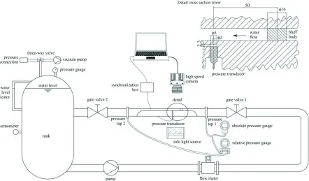
The experimental setup in Fig. 1 was used for the experiment. It consists of cavitation station with cavitation test section and measurement equipment. It is more thoroughly discussed in the following subsections.
1.1 Cavitation Station
Cavitation station is shown in Fig. 1. The main elements of cavitation station are water tank, main circulation pump, vacuum pump, cavitation test section and measurement equipment for cavitation station operational point regulation.
The quantity of water in the cavitation station
was approximately 1 m3. It was driven by a radial
circulation pump. Unprepared tap water was used for the experiments. Water quality was not measured, but we replaced the water in the cavitation station prior to measurements with fresh tap water. Operating pressure in the system was set by a vacuum pump through a three way valve at the top of the water tank.
Measurement equipment for cavitation station operating point selection comprised of pressure and volume flow rate measurement equipment. Operating pressure was measured with absolute pressure transmitter ABB 2600T Series 264 VS. Pressure drop on the test section was measured with absolute pressure transmitter ABB 2600T Series 264DS. Four pressure taps were located upstream and downstream of the test section. The uncertainty of the operating pressure measurement was estimated to ±0.5% of measured value.
Volumetric flow rate was measured with electromagnetic flow meter ABB COPA-XL DL43F DN 125/PN 16. The measurement uncertainty of volumetric flow rate was up to ±1% of measured value. The experiment was performed with water
temperature close to ambient temperature (T = 24
°C). Water temperature was measured with Pt100 thermometer mounted inside the water tank and connected to Agilent 34970A data acquisition unit. Temperature measurement uncertainty was estimated to ±0.5 °C.
1.2 Test Section
Cavitation station test section is shown in Fig. 1. The test section dimensions were 50 mm (width) × 10 mm (height) × 800 mm (length). Pressure pulsations were generated by a bluff body with diameter of 16 mm. The height of the bluff body was the same as the height of the test section. The bluff body was manufactured from hard rubber and was compressed and held in place by wall friction. No cavitation was observed near the junction of the bluff body and test section wall. The bluff body was mounted 50 mm upstream from the pressure transmitter.
Measurement equipment consisted of a fast pres-sure transmitter and a high speed camera.
Pressure oscillations were measured with PCB Piezotronics pressure transmitter type 111A26 with frequency range from 0.01 Hz to 400 kHz and dynamic pressure range of 34.5 bar. The transmitter was mounted to the wall of the cavitation test section as shown in Fig. 1. The pressure transmitter was mounted in an insert, which was flush mounted to the test section lower wall. The transmitter was connected to the test section through a hole 3 mm in length and 2 mm in diameter and a cavity 2 mm in length and 5 mm in diameter, as shown in Fig. 1. The transmitter was protected against cavitation erosion with the above mentioned installation installation. Power to the transmitter was supplied using PCB Piezotronics 480C02 signal conditioner. The signal conditioner has a frequency range from 0.05 to 500 kHz. Pressure was acquired with 16 bit data acquisition board national Instruments NI-USB 6351 with 1.25 MHz sample rate. The convenient roll-off of the signal conditioner and selected frequency of acquisition enabled operation without aliasing filters. The duration of acquisition was 2 s. Data was stored to the disk immediately after the acquisition.
a distance 20 cm parallel to the cavitation station test section wall. A 70 mm cylindrical lens was attached to LED lights. It was used to focus illumination on a light sheet with thickness of approximately the same size as the height of water above the pressure transmitter. The entire distance from the bluff body to the pressure transmitter was uniformly illuminated. Such installation also prevented any unwanted reflections and provided very strong illumination required by the short shutter time.
Pressure and image acquisition was synchronized with the trigger from an electronic synchronization device. The trigger started the acquisition; later acquisition timing was performed using internal clocks of the data acquisition board and the camera.
1.3 Image Processing and Void Fraction Estimation
The high speed camera acquired series of eight-bit greyscale images that were showing cavitation inside the cavitation test section. For image post-processing image with pixels can be presented as a matrix with elements. Eight-bit resolution gives 256 levels of greyness A(i, j, n), which the matrix element can occupy (0 for black pixel and 255 for white pixel)
A(i, j, n) ∈ {0,1,…, 255}. Each image is thus presented as a matrix:
Image n
A n A I n
A J n A I J n
( )
= … … ( , , ) ( , , ) ( , , ) ( , , ) .1 1 1
1
M O M (1)
For the evaluation of brightness µ of a region of interest we averaged brightness of the pixels in the region of interest (ROI) [20]:
µ n
IROI JROI A i j n
( )
=⋅
∑∑
1 ( , , ). (2)
Although the exact relationship between the of
cavitation clouds void fraction A and average ROI
brightness µ cannot be established with single BW
camera and present image acquisition configuration, we assumed that cavitation cloud void fraction
A is proportional to the brightness µ in a ROI
corresponding to a cavitation cloud:
A n( )∝µ( ).n (3)
This estimation is valid under the assumption that cavitation clouds are white, uniformly illuminated and that no reflections are recorded on them. We also
did not take into consideration the shape of cavitation clouds, which has a major influence on the cavitation cloud void fraction. While the above procedure provided useful results, other measurement methods give better estimation of void fraction. Among them is x-ray computed tomography measurement [16] or time resolved 2D X-ray densitometry [21] method.
A rectangular region of interest was used as shown in Fig. 2. We used the size of ROI 65×65 pixels which corresponds to 10.4×10.4 mm. The pressure transducer hole was located in the same position as the center of ROI. All sets of images were analyzed with ROI of the same size and position.
Fig. 2. The region of interest (ROI) in the wake of bluff body
Value of estimated void fraction was normalized in every operating point, such that the void fraction value 0 represents the lowest measured ROI brightness
µ and void fraction value 1 represents the highest
measured ROI brightness µ. Such normalization was
performed in each operating point.
2 THE RESULTS
The cavitating flow characteristics were observed at three different operating conditions with different cavitation cloud dynamics. The operating conditions
are related to the cavitation number value σ and are presented in Table 1. The cavitation number σ was
used as follows:
σ ρ = − ∞ p p U ref v l 1 2 2
, (4)
where pref is reference pressure in the cavitation
station, pv is vapour pressure, ρl is density of water and U is water velocity.
OP1 t = 1815 ms OP1 t = 1816 ms OP1 t = 1817 ms OP1 t = 1818 ms OP1 t = 1819 ms
OP2 t = 1759 ms OP2 t = 1760 ms OP2 t = 1761 ms OP2 t = 1762 ms OP2 t = 1763 ms
OP3 t = 1822 ms OP3 t = 1823 ms OP3 t = 1824 ms OP3 t = 1825 ms OP3 t = 1826 ms
Fig. 3. Images of cavitation in the wake of bluff body for three operating points
the cavitation cloud shedding length and void fraction (brightness) in the wake. The phenomenon shows periodic nature for all operating points.
Table 1. Selection of operating points
Operational point OP1 OP2 OP3
Reference pressure [bar] 1.50 1.44 1.40 Flowrate [m3/h] 19.8 19.6 19.5 Cavitation number 1.31 1.26 1.22
In the following subsection we will present time series of measured variables, corresponding power spectra and amplitude demodulation analysis.
2.1 Time Series Analysis
Time series show time evolution of analyzed variables.
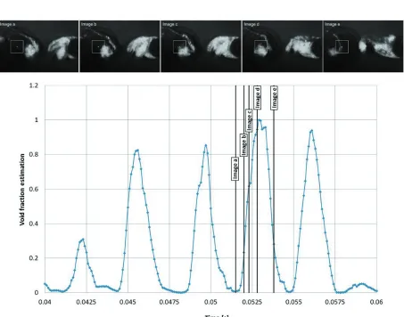
A sample time series of void fraction A is shown in
Fig. 4. In addition one period of cavitation cloud shedding is accompanied with corresponding images of the phenomenon. The rectangular frame in Fig. 4
shows the location of ROI where void fraction A was
estimated for each picture in the series. Void fraction fluctuates when cavitation structure passes the ROI.
In Fig. 4, subimage a shows no cavitation cloud in the ROI and void fraction is low. Images b and c show an increase of cavitation cloud in the ROI, while void fraction increases. Image d shows approximately the highest amount of cavitation in the ROI; here void
OPI 1
a) b)
OPI 2
c) d)
OPI 3
e) f)
fraction is the highest. In image e cavitation cloud left the ROI and void fraction decreased.
We now compare void fraction A estimation time
series with pressure p measurements time series. Both
variables were simultaneously acquired and recorded at the same distance from bluff body (Fig. 2). Pressure transducer hole is located in the same position as the
center of the ROI. Fig. 5 shows pressure p(t) and
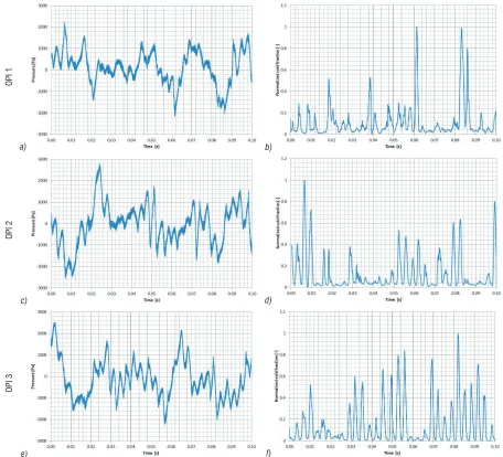
void fraction A(t) time series for operational points OP1 to OP3. Both variables show periodic behavior for all operating points. Pressure measurements show fluctuations of low frequency, while high frequency pressure fluctuations are imposed upon low frequency content. The low frequency pressure fluctuations correspond to cavitation cloud shedding and their passage across the ROI.
Local pressure fluctuations and cavitation bubble collapses near the pressure transducer sensing hole contribute more to the measured pressure, while there is no equivalent of this information in the void fraction estimation.
Void fraction fluctuations show only low frequency fluctuations. Estimation of void fraction at high frequencies was not possible due to low camera acquisition speed of 10 kHz and spatial averaging, introduced by a large ROI. If we analyze the influence of cavitation number on the void fraction fluctuations, we can see that in the operating point OP1 and to a lesser extent also OP2 the number of peaks decreases (comparing Figs. 7b, d and f).
OPI 1
a) b)
OPI 2
c) d)
OPI 3
e) f)
2.2 Signals in Low Frequency Domain
Fig. 6 shows the unfiltered pressure and void fraction spectra in the low frequency domain. Several peaks of fluctuations show periodic behavior of pressure and void fraction in the region bellow 1 kHz. Among them are frequency peaks at 30 and 310 Hz in the pressure spectra and void fraction spectra. Pressure and existence of void fraction are closely connected. In the case of OP1, which corresponds to the highest cavitation number, there are few significant frequencies in pressure or void fraction power spectra.
As shown in Fig. 6, periodic shedding of vortices from the bluff body is responsible for frequency peaks around 310 Hz. Peaks around 310 Hz in pressure spectra and in void fraction exactly match in frequency.
We assume that unsteady flow behavior inside the cavitation station is responsible for measured pressure fluctuations with peaks around 30 Hz. The presumption of flow driven fluctuations at 30 Hz seems to be confirmed with the amplitudes of peaks at 30 Hz which do not follow cavitation intensity in an individual operating point (Figs. 6c and e).
Pressure fluctuations are also represented in void fraction fluctuations, which follow pressure fluctuations with the same frequency.
In accordance with Eq. (4), the amplitude of peaks at 310 Hz frequency domain for both signals decreases with the intensity of cavitation.
In general, Strouhal number is used to describe unsteady and oscillating flow problems. It is defined as the ratio of inertial forces due to the unsteadiness of the flow or local acceleration to the inertial forces due to changes in velocity from one point to another in the flow.
St f d
v
= × .
In our case the flowrate was nearly the same for analyzed operating points (Table 1). According to cavitation fluctuations frequency (310 Hz), bluff body diameter (16 mm) and cavitation section surface area (5×10⁻⁴ m2) the value of Strouhal number was constant
(St = 0.45) regardless of the cavitation number value.
2.3. High Frequency Analysis and Amplitude Demodulation of High Pressure Fluctuations
The study of high frequency vibrations and pressure fluctuations is a known technique of cavitation analysis [18]. The frequency analysis of pressure time series was performed in the high frequency range
with band pass filtering ranging from 300 to 400 kHz. Due to the recessed installation of pressure sensor as explained in section 1, pressure signal was damped in comparison with flush mounting installation. We estimated that damping in the selected frequency interval was around –10 dB.
The 4th order Butterworth filter was used
for signal conditioning. It is known that the high frequency spectral content of pressure fluctuations cannot solely be attributed to cavitation. Other flow excitations, bearing friction, vibrations, rubbing etc. may excite high frequency pressure fluctuation. To address this problem, the amplitude demodulation technique was applied for improved signal analysis in a cavitation tunnel [22] and in a prototype turbine model by Escaler et al. [23].
The Strouhal frequency related to the natural frequency of two phase flow interacted with flow induced pulses can be determined using the amplitude demodulation technique as shown by Abbot et al. [22], Farhat et al. [24], Callenaere et al. [25] and Escaler et al. [22] and [26].
In our case, pressure pulsations were measured in a broad frequency interval. We were able to record low pressure fluctuations as shown in Fig. 6. These correspond to the frequency of cavitation clouds shedding from the bluff body (Fig. 4).
We will now discuss the connection between low frequency fluctuations and amplitude demodulation of very high frequency pressure fluctuations. The cavitation cloud that travels above the pressure sensor produces very high frequency pressure fluctuations in the frequency range of several 100 kHz. These fluctuations may be a result of local cavitation bubble collapses. The latter, however, appear only when the cavitation cloud is present near the pressure transducer. We can identify low frequency pressure pulsations using amplitude demodulation technique of local cavitation bubble collapses which appear in the very high frequency range. In the frequency domain, amplitude demodulation permits identification of frequencies associated to the dynamic behavior of the cavitation clouds. In our case, this corresponds to cavitation cloud periodic shedding. In the case of cavitation in turbine machinery runner, the cavitation can be identified at a modulated frequency of a particular hydrodynamic phenomenon [23].
of the Hilbert transform with the aid of fast Fourier transform (FFT) routines. In order to simplify, the continuous Hilbert transform is written as follows:
H p t p
t d
( ( )) ( ) ( ) . =
−
−∞ ∞
∫
1 π
τ
τ τ (5)
In the third and last step, low frequency amplitude envelope of the filtered high frequency signal is created. In our case of pressure fluctuations the amplitude demodulation was calculated as:
ADM t( )= H p t
(
( )
)
2+p t( )
2. (6)Signal processing was performed using Labview fast Hilbert transform virtual instrument subroutine. The resulting filtered amplitude demodulated envelope is shown in Figs. 7 a, c and e.
The spectral analysis of the amplitude demodulated pressure is shown in Figs. 7, b, d and f.
Filtered and amplitude demodulated envelopes of very high frequency pressure fluctuations show periodic pulsating nature, which is connected to the cavitation cloud shedding at the bluff body. The spectral analysis in Figs. 6, b, d and f shows peaks around the frequency of 310 Hz with increasing amplitudes in the cavitation more intensive operating regimes. This statement confirms that traveling
OPI 1
a) b)
OPI 2
c) d)
OPI 3
e) f)
cavitating clouds produce high frequency pressure fluctuations which correspond to local cavitation bubble implosions. Using the amplitude demodulation technique, these high frequency pulsations can be transformed to periodic pulsations at lower frequencies which are associated with the dynamic behavior of cavitation clouds. In our case, the envelope pulsation frequency directly corresponds to the shedding of cavitation vortices from the bluff body. The correlation is expressive for the regimes where Von Karman structures in the wake reach the position of the pressure sensor.
3 CONCLUDING REMARKS
The simultaneous study of cavitation cloud dynamics and corresponding pressure pulsations in the cavitation station was presented in the paper. Cloud cavitation takes place in the external flow and initiates periodic pressure fluctuations. Unsteady flow nature with collapsing cavitation clouds follows the vortex shedding process with Von Karman type structures in the wake of the submerged bluff body, while cavitation intensity does not affect the Strouhal number value.
The present investigation shows strong interaction between pressure and cavitation cloud structure dynamics. The similarity between high speed camera and pressure transmitter signals was observed in time and frequency domain. The study shows two dominant frequency bands, connected to cavitation cloud structure passing the area of interest and cavitation dynamics within the cloud. The low frequency cavitation instabilities show a connection to high frequency dynamics inside cavitation clouds when cavities in the Von Karman structure reach the position of pressure and cavitation cloud structure sensing.
For further study, much higher speed and resolution of the image acquisition system and flush mounted pressure transmitter is preferred for more detailed analysis of cavitation clouds and interaction of pressure fluctuations.
4 REFERENCES
[1] Singhal, A.K., Athavale, M.M., Li H., Jiang, Y., (2002). Mathematical basis and validation of the full cavitation model. Journal of Fluids Engineering, vol. 124, no. 3 p. 617-624, DOI:10.1115/1.1486223.
[2] Biluš I., Morgut M., Nobile E. (2013). Simulation of Sheet and Cloud Cavitation with Homogenous Transport Models. International Journal of Simulation Modelling, vol. 12, no. 2, p. 94-106, DOI:10.2507/ IJSIMM12(2)3.229.
[3] Dular, M., Coutier-Delgosha, O., (2009). Numerical modelling of cavitation erosion. International Journal for Numerical Methods in Fluids, vol. 61, no. 12, p. 1388-1410, DOI:10.1002/fld.2003.
[4] Wade, R.B., Acosta, A.J. (1966). Experimental observation on the flow past a plano-convex hydrofoil. Transaction of ASME, Journal of Basic Engineering, vol. 87, no. 1, p. 273-283, DOI:10.1115/1.3645829. [5] Kjeldsen, M., Arndt, R.E.A., Effertz, M. (1999).
Investigation of unsteady cavitation phenomena. Proceedings of the 3rd ASME/JSME Fluids Engineering
Conference, San Francisco.
[6] George, D.L., Iyer, C.O., Ceccio, S.L. (2000). Measurement of the bubbly flow beneath partial attached cavities using electrical impedance probes. Journal of Fluids Engineering, vol. 122, no. 1, p. 151-155, DOI:10.1115/1.483237.
[7] Kubota, A., Kato, H., Yamaguchi, H., Maeda, M. (1999). Unsteady structure measurement of cloud cavitation on a foil section using conditional sampling technique. Journal of Fluids Engineering, vol. 111, no. 2, p. 204-210, DOI:10.1115/1.3243624.
[8] Reisman, G.E., Brennen, C.E. (1996). Pressure pulses generated by cloud cavitation. ASME Fluids Engineering Division Conference, San Diego.
[9] Brandner, P.A., Walker, G.J., Niekamp, P.N., Anderson, B. (2007). An investigation of cloud cavitation about a sphere. 16th Australasian Fluid Mechanics Conference,
Crown Plaza.
[10] Reisman, G. E.,Wang, Y.C., Brennen, C.E. (1998). Observations of shock waves in cloud cavitation. Journal of Fluid Mechanics, vol. 355, no. 1, p. 255-283, DOI:10.1017/S0022112097007830.
[11] Langa, S., Dimitrov, M., Pelz, P.F. (2012). Spatial and temporal high resolution measurement of bubble impacts. 8th International Symposium on Cavitation,
Singapore, DOI:10.3850/978-981-07-2826-7_210 [12] Keil, T., Pelz, P.F., Cordes, U., Ludwig, G. (2011).
Cloud cavitation and cavitation erosion in convergent divergent nozzle. WIMRC 3rd International Cavitation
Forum, Coventry.
[13] Van Terwisga, T.J.C., Fitzsimmons, P.A., Ziru, L., Foeth, E.J. (2009). Cavitation Erosion – A review of physical mechanisms and erosion risk models. 7th
International Symposium on Cavitation, Ann Arbor. [14] Heath, D., Širok, B., Hočevar, M., & Pečnik, B. (2013).
The use of the cavitation effect in the mitigation of CaCO3 deposits. Strojniški vestnik - Journal of Mechanical Engineering, vol. 59, no. 4, p. 203-215, DOI:10.5545/sv-jme.2012.732.
[15] Leppinen, D.M., Dalziel, S.B. (2001). A light attenuation technique for void fraction measurement of microbubbles. Experiments in Fluids, vol. 30, no. 2, p. 214-220, DOI:10.1007/s003480000158.
Fluids, vol. 54, no. 7, p. 1-21, DOI:10.1007/s00348-013-1561-z.
[17] Bauer, D., Chaves, H., Arcoumanis, C. (2012). Measurements of void fraction distribution in cavitating pipe flow using x-ray CT. Measurement Science and Technology, vol. 23, no. 5, p. 10, DOI:10.1088/0957-0233/23/5/055302.
[18] Maurus, R., Ilchenko, V., Sattelmayer, T. (2002). Study of the bubble characteristics and the local void fraction in subcooled flow boiling using digital imaging and analysing techniques. Journal of Experimental Thermal and Fluid Science, vol. 26, no. 1, p. 147-155, DOI:10.1016/S0894-1777(02)00121-8.
[19] Iyer, C.O., Ceccio, S.L. (2002). The influence of developed cavitation on the flow of a turbulent shear layer. Physics of Fluids, vol. 14, no. 10, p. 3414-3431, DOI:10.1063/1.1501541.
[20] Osterman, A., Hočevar, M., Širok, B., Dular, M. (2009). Characterization of incipient cavitation in axial valve by hydrophone and visualization. Experimental Thermal and Fluid Science, vol. 33, no. 4, p. 620-629, DOI:10.1016/j.expthermflusci.2008.12.008.
[21] Makiharju, S., Ganesh, H., Ceccio, S. (2012). Time resolved 2D X-ray densitometry of a cavitating wedge. Bulletin of the American Physical Society, 65th Annual
Meeting of the APS Division of Fluid Dynamics, San Diego.
[22] Abbot, P.A., Arndt, R.E.A., Shanahan, T.B. (1993). Modulation noise analyses of cavitating hydrofoils. ASME-FED Winter annual meeting, Bubble Noise and Cavitation Erosion in Fluid Systems, vol. 176, p. 83-94. [23] Escaler, X., Egusquiza, E., Farhat, M., Avellan, F.,
Coussirat, M. (2006). Detection of cavitation in hydraulic turbines. Mechanical Systems and Signal Processing, vol. 20, no.4, p. 983-1007, DOI: 10.1016/j. ymssp.2004.08.006.
[24] Farhat, M., Avellan, F., Pereira, F. (1992). Pressure fluctuations downstream a leading edge cavity. La Houille Blanche, vol. 47, no. 7/8, p. 579-585, DOI:10.1051/lhb/1992061. (in French)
[25] Callenaere, M., Franc, J.P., Michel, J.M., Riondet, M. (2001). The cavitation instability induced by the development of a reentrant jet. Journal of Fluid Mechanics, vol. 444, no. 1, p. 223-256, DOI:10.1017/ S0022112001005420.