Spatial-Mode-Shape Identification using a Continuous
Wavelet Transform
Martin Česnik - Janko Slavič - Miha Boltežar*
University of Ljubljana, Faculty of Mechanical Engineering, Ljubljana, Slovenia
This paper presents an experimental modal analysis of a damped multi-degree-of-freedom mechanical system using a continuous wavelet transform. An approximation of the wavelet transform of the impulse response function is deduced, which serves as a basis for the extraction of the natural frequencies, the damping ratios and the mode shapes. Due to an approximation with a finite Taylor series, a computational error in the identified oscillatory amplitude occurs and is observed for the simulated system response. The presented approach of modal identification is applied to real mechanical systems, such as a steel beam and the horizontal tail of an ultralight aircraft. Using the proposed measurement methodology, it is possible to reconstruct the spatial mode shapes of any dynamic linear system with an arbitrary geometry.
© 2009 Journal of Mechanical Engineering. All rights reserved.
Keywords: modal parameters, continuous wavelet transform, spatial vibrations
0 INTRODUCTION
One of the key steps in the development of a numerical model is its validation, where the modal analysis of a numerical model and the experimental modal analysis (EMA) of the real system are compared. With the results of the comparison it is possible to determine the adequateness of the numerical model.
The most common way to undertake a modal analysis is by measuring the frequency response-functions (FRF) [1] and [2]. This is done by signal transformation from the time domain to the frequency domain using a Fourier transformation. With the use of a fast Fourier transform (FFT) algorithm, the calculation of the FRF is a simple and useful method used to perform an EMA [3] to [5]. The described method is suitable for analyzing stationary signals, since it averages the signal in time domain. For an analysis of non-stationary signals it is convenient to use transformations in the time or time-frequency domain, for instance, least-squares complex exponential (LSCE) [1], continuous wavelet transform (CWT) [6], etc.
The impulse response of a mechanical system is a typical non-stationary process where the oscillation amplitude decreases exponentially with time. Generally, the modal identification, based on non-stationary signals, is usually done with time-domain methods [1], e.g. LSCE for impulse response function or Ibrahim time
domain (ITD) for free decay response. The idea of applying a CWT to a dynamic system response for damping identification was first introduced by Staszewski [7]. While Staszewski used the Morlet wavelet function, Slavič et al. [8] to [10] developed their idea using the Gabor wavelet function and focusing it on the edge effect and the relatively short signals. The properties of the Gabor wavelet have been studied in detail by Simonovski and Boltežar [11], who also used it for fault detection in DC electro-motors [12].
Le and Argoul [13] extended the work of precendent researchers and identified all the modal parameters by applying a CWT to the theoretical impulse response of a spatial 4-degree-of-freedom (DOF) model with the Morlet, Cauchy and harmonic wavelet functions. They also explored the problem of the edge-effect and time-frequency localization.
mode shapes by a determination of the planar displacements in a horizontal plane.
To continue their work, Česnik et al. [16] tried to extract the spatial mode shapes of a mechanical system with an arbitrary geometry. This work represents a continuation and enhancement of that research.
In this paper, a procedure for the identification of the modal parameters is introduced, based on a CWT of the impulse response function. Due to the low-order approximation, a computation error of the oscillatory amplitude occurs when dealing with systems with high damping, which is presented in a numerical example. The method is also tested on a real system of a steel beam The method is also tested on a real system of a steel beam where the estimated mode shapes are compared with the theoretical ones. With the identification of the spatial mode shapes of the horizontal tail of an ultralight aircraft, the feasibility of the developed method is proven.
1 CONTINUOUS WAVELET TRANSFORM The introductory part of CWT theory will be summarized according to Mallat [6] and Tchamitchian et al. [17]. The continuous wavelet transformation of the time function f(t), that satisfies f(t)∈L2(ℜ)
is defined as *
,
( , ) ( ) u s( ) d ,
Wf u s f t
ψ
t t+∞
−∞
=
∫
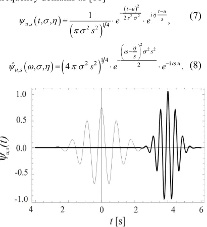
⋅ (1) where ψ(t) represents the wavelet function, the superscript * denotes the complex conjugate, u is the translation parameter related totime and s is the scale parameter that serves as an inverse of the frequency. Fig. 1 shows the influence of the parameters u and s on the wavelet function.
The function f(t)∈L2(ℜ)may be treated
as a mother wavelet function when satisfying oscillatory, energy preservation and admissibility conditions [6]. A modified wavelet function ψu,s(t), translated in the time domain and dilated
in the frequency domain also has to satisfy the energy-preservation condition, and so we obtain
( )
, 1 , u s t u t s s ψ = ⋅ ⎜ψ⎛ − ⎞⎟⎝ ⎠ (2)
( )
i( )
,
ˆ u ˆ ,
u s s e ω s
ψ ω = ⋅ − ⋅ ⋅ ⋅ψ ω (3)
where ψˆu s, ( )ω denotes the integral Fourier transformation of the wavelet function ψu,s(t) in
the frequency domain.
The impulse response of a multi-degree-of-freedom (MDOF) system is expected to be a summation of N mutually independent function pairs [7]
( )
( )
i ( )1 , i N t i i
f t A t eϕ
=
=
∑
(4)where Ai(t) denotes the amplitude and
ϕi(t) the phase (9). Therefore, the linearity
property of the CWT [6] can be used
( )
( )( )
1 1
, , .
N N
i i i i
i i
W α f u s α Wf u s
= = ⎛ ⎞ = ⎜ ⎟ ⎝
∑
⎠∑
(5)1.1 Gabor Wavelet Function
The Gabor mother wavelet function is defined as [6]
( )
( )
2 2 i 2 1 4 2 1 , , . t tGabor t e σ eη
ψ σ η
π σ
−
= ⋅ ⋅ (6)
By introducing the translation and dilation parameters into (6), we obtain a family of Gabor wavelet functions, defined in the time and frequency domains as [11]
(
)
(
)
( )2 2 2 i
2
, 2 2 1 4
1
, , ,
t u t u
s s
u s t e e
s η σ ψ σ η π σ − − −
= ⋅ ⋅ (7)
(
)
(
)
2 2 2
1 4
2 2 2 i
,
ˆ , , 4 .
s s
u
u s s e e
η ω σ ω ψ ω σ η π σ ⎛ − ⎞ ⎜ ⎟ ⎝ ⎠ − −
= ⋅ ⋅ (8)
Fig. 1. (─) mother ψGabor
(
t u, =0, s=1)
and1.2 Approximation of the CWT of the Asymptotic Function
The impulse response of a viscously damped single-degree-of-freedom (SDOF) system can be written as [8]
( )
0(
)
0d 0
cos ,
t
f t =A e−ζ ω ⋅ ω t+ϕ (9) where ζ denotes the damping ratio, ϕ0 is the
phase shift, ω0 is the undamped angular
frequency and 2
0d 0 1
ω =ω −ζ is the damped angular frequency. In order to separate the amplitude and the phase information of the response function it can be written in a more general form as an analytic function [17]
( )
( )
i ( ). f t
a f
f t =A t eϕ (10) Similarly, a wavelet function may also be given in the form of an analytic function as
( )
( )
i ( )ta t A t e ψ
ϕ ψ
ψ = ⋅ . With regards to the relation
( ), 1 2 a( ),
Wf u s = ⋅Wf u s [6] we can deduce that
( )
( ) i 1 ( , ) 2 d . f f t u t s t uWf u s A t A
s
e ψ t
ψ ϕ ϕ +∞ −∞ ⎛ − ⎛ − ⎞⎞ ⎜ ⎜⎝ ⎟⎠⎟ ⎝ ⎠ − ⎛ ⎞ = ⋅ ⎜ ⎟ ⎝ ⎠ ⋅
∫
(11)In order to solve the equation (11), a few approximations have to be made: the function
Sf(t) is approximated with a zero-order Taylor
series (i.e., a constant value A), and the function ϕf(t) is approximated with a first-order Taylor
series. By using these approximations, a general solution of the CWT can be deduced [8]
( )
( )(
( )
)
( )
( )
(
)
i 1 ˆ ( , ) ' , , 2 '' , ' , f u f f f fWf u s A u e u
Er A u u
ϕ ψ ϕ η σ
ϕ
= ⋅ ⋅
+ (12)
where Er A
(
f ''( )
u ,ϕf '( )
u)
denotes the error function due to the use of the finite Taylor series. On the basis of the linearity property of the CWT (5) we can apply an approximation (12) to multi-component functions, such as the impulse response of the MDOF system (4) in order to identify the modal parameters of a particular natural frequency.1.3 Modal Parameter Identification
Due to the nature of a CWT it is possible to transform the measured signal in form of a time series to the frequency domain without the loss of time-domain information. Furthermore, a CWT offers very good resistance to the noise in the measured signal. Regarding the nature of the CWT, it is possible to observe the development of natural frequencies with time. In order to apply the CWT to modal analysis it is essential to analytically describe the distinctive properties of the impulse response’s wavelet transformation. The deduction of the impulse-response CWT will be presented according to Staszewski [7] and Slavič [8], who analyzed the Morlet and Gabor wavelets, respectively.
From equation (11) we can see that the essential contribution to the magnitude is provided by the stationary points of the argument of the integrand [16], i.e., the points ts, such that
'
( )
1 ' s .f s
t u
t
s ψ s
ϕ
=ϕ
⎛⎜ − ⎞⎟⎝ ⎠ (13)
The canonical pairs
( )
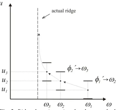
u s, , which satisfy the condition ts(u,s)=u define the ridge of thewavelet transform [17]. The ridge can be detected with different approaches, and Staszewski presented three: the cross-section method, the amplitude method and the phase method [7]. In this work, the phase method, which is based on a frequency match (13), is used. In order to determine the ridge an initial estimation of the instantaneous frequency ω1 has to be made. It is
then entered into the recursive equation
1
(
1) (
1)
1 1
, ,
,
i i i i
i i i u u u u
φ
η ω
φ
η ω
ω
+ − + + − − =− (14)
which gradually converges to an instantaneous frequency in the signal (Fig.2).
The values of the wavelet transform restricted to its ridge are called the skeleton of the wavelet transform; they serve for the modal-parameter identification (16, 17).
Fig. 2. Ridge detection using the phase method with the recursive equation (14)
Due to the linear relation between frequency and scale for the Gabor wavelet φ'(u,s)=η/s we can conclude that the scale variable on the ridge
s(u)is constant s(u)=s0.
By introducing the Gabor wavelet function into equation (12), regarding the frequency match and neglecting the error function, it follows that [6]
(
)
0d(
2 2)
1 40 0
1
, 4 .
2
u
Wf u s = Ae−ζ ω π σ s (15)
Finally, we can deduce equations for the direct identification of the damping ratio ζ and the initial amplitude A
(
)
(
0)
0d
ln ,
const.,
Wf u s u ζ
ω ∂
∂
= − ≈ (16)
(
)
(
)
(
)
0d
0 1 4 2 2
0d
2 ,
const. 4
u
e Wf u s
A ζ ω
π σ η ω
= ≈ (17)
1.4 A t
( )
Variation Influence on the Identified AmplitudeAn approximation for the theoretical CWT of the impulse response is deduced by approximating an impulse response (9) as a finite Taylor series. An approximation of A(t) = const. is exact only for asymptotic signals, like the undamped response, where the phase variations are considerably faster than the amplitude variations
( )
( )
( )
'
' .
f
f f
A t
t
A t <<ϕ (18)
When considering signals by which the asymptotic condition is not entirely satisfied, e.g., a highly damped impulse response, an error occurs during the amplitude A identification.
The presented error represents a deviation of the reconstructed amplitude Areconstr
from the real amplitude in the system response
Areal. It can be observed from a numerical
example of a highly damped impulse response and depends on the damping ratio ζ and the parameter σ (Fig. 3 and Fig. 4); however, it is independent of the real amplitude value Areal.
Consequently, the ratio between the real amplitude Areal and the reconstructed amplitude Areconstr which serves for the mode-shape
reconstruction, is constant 1 real 2 real
1 reconstr 2 reconstr
const.
A A
A = A = (19)
Fig. 3. Reconstructed initial amplitude at variable parameter σ and Areal(t = 0) =1.
Fig. 4. Reconstructed initial amplitude at
(
)
1 real 0 1
This finding is important when a reconstruction of the mode shape is made only by comparing the amplitudes of the displacements at different measurement positions (Section 2.1). 1.5 Spatial Mode Shapes – Geometry
In order to reconstruct the spatial mode shapes the spatial vibrations have to be measured with accelerometers at pre-defined measurement positions. When performing a modal analysis on simple geometry such as a steel beam (Section 2.1), the response accelerometers can be oriented in the same direction and no issues arise from the geometry point of view. When analyzing a system with three-dimensional geometry, the orientation of the response accelerometers in the same direction as the reference one is not always possible (Fig. 5). To overcome this problem, the local coordinate system of each accelerometer is referenced to the global coordinate system of the measured sample.
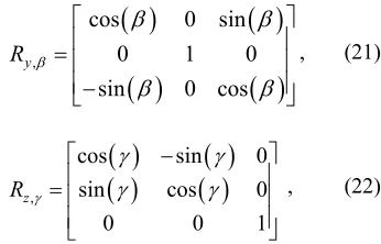
One possibility of describing this linkage is with the Euler angles (Eqs. 20 to 22).
Fig. 5. Problem of spatial vibration measurements
To reconstruct a single spatial mode shape, the identified displacements need to be transformed from the local coordinate systems (as measured) into the global coordinate system with the use of the rotational matrices
( )
( )
( )
( )
,
1 0 0
0 cos sin
0 sin cos
x
R α α α
α α
⎡ ⎤
⎢ ⎥
=⎢ − ⎥
⎢ ⎥
⎣ ⎦
, (20)
( )
( )
( )
( )
,
cos 0 sin
0 1 0
sin 0 cos
y
R β
β β
β β
⎡ ⎤
⎢ ⎥
= ⎢ ⎥
⎢− ⎥
⎣ ⎦
, (21)
( )
( )
( )
( )
,
cos sin 0
sin cos 0
0 0 1
z
R γ
γ γ
γ γ
⎡ − ⎤
⎢ ⎥
= ⎢ ⎥
⎢ ⎥
⎣ ⎦
, (22)
where α, β and γdenote the Euler rotation angles about the x, y or z axis, respectively.
1.6 Identification of the Spatial Mode Shapes
The procedure to perform the experiment and reconstruct the single spatial mode shape is presented in the following steps:
a) Experiment
1. Definition of the excitation position. 2. Definition of the global coordinate
system, n response positions with n local coordinate systems on the measured sample’s geometry.
3. Selection of the reference position and the reference direction (this should be the position/direction where high oscillations of the identified modes are expected).
4. Excitation of the system with the impulse hammer, acceleration measurement on the reference position/direction and on the response position(s) in the chosen direction(s).
b) Reconstruction
5. Identification of the ridge (14) and of the initial amplitudes Aref,j and Aresp,i,j (17) for
the reference and response signals, respectively; j denotes the consecutive number of the impulse excitation and i is the number of the response position (i=1,…, n).
6. Computation of the normalized response amplitude Anorm,i with respect to the
7. Transformation of the normalized displacements Anorm,i from the local to the
global coordinate system (Eqs. 20 to 22). 8. Graphical presentation of the
spatial-mode shape.
2 EXPERIMENT
For a relatively simple steel beam, the presented approach for modal identification is experimentally compared to the beam’s theoretical mode shapes. Furthermore, to demonstrate an experimental identification of the spatial modal analysis, the horizontal tail of an ultralight aircraft is presented.
2.1 Experimental Validation
In order to perform a specific numerical manipulation, custom programs and algorithms were developed by the authors. Custom-made programs offer a higher flexibility and provide the author with an insight into the computation process. To check the correctness of the developed programs a simple experiment with well-defined theoretical mode shapes was carried out. With algorithms that are verified on simple models, it is possible to perform a reliable modal analysis on more complex spatial structures.
A simple validation experiment for method verification was performed on a free-free supported steel beam with dimensions of 5x40x1000 mm, excited by an impulse hammer at a pre-defined "excitation" position. The experiment was made with several impulse excitations; during each excitation the response accelerometer was at a different position, as described in the following.
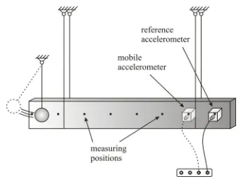
For the sake of experimental simplicity, only two accelerometers were used for the measurements. One accelerometer was denoted as the "reference" sensor and was always placed in the "reference" position. The second accelerometer, denoted as the "response" accelerometer was placed at a different "response" position during each impulse excitation.
When carrying out the described experimental procedure a precaution should be taken; due to changing of position of the response accelerometer a mass matrix of the whole beam
system is changing. As a result some errors of the reconstructed mode shapes and belonging natural frequencies could occur, especially when using accelerometers with considerable mass and when identifying high-order mode shapes with local nature. With application of a lightweight accelerometer with a mass of 1g and at identification of global mode shapes only negligible errors are expected at the validation experiment.
Eleven measuring positions were set along the beam: position 1 was defined as the "reference" position, and the remaining positions were defined as the "response" positions, as shown in Fig. 6.
Fig. 6. Measuring-position placement on the analyzed beam
After the whole set of measurements was carried out, we could obtain the impulse response from any pre-defined position along the beam.
Fig. 7. The validation-experiment configuration set-up
With the use of a CWT on the measured responses it is possible to identify the modal parameters according to the theoretical backgrounddescribed in Section 1.3. The Eq. (14) is used to define the time development of an observed natural frequency. Once the value of the natural frequency is known, Eqs. (16) and (17) are used to define the damping ratio ζ of the system and the initial amplitude A at the location of the measurement.
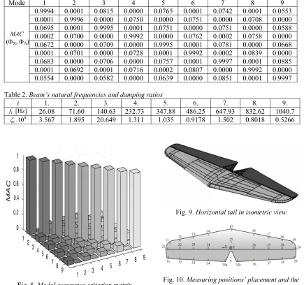
positions (Section 1.6), the first nine normalized mode shapes were reconstructed and compared to the theoretical mode shape by computing the Modal Assurance Criterion MAC (ΦX, ΦA) [1],
shown in Figure 8 and stated in Table 1. Table 2 shows the associated natural frequencies fi and
the damping ratios ζi.
2.2 Horizontal Tail Experiment
An experiment similar to the one described in Section 2.1. was carried out on the horizontal tail of an ultralight aircraft. Since the tail geometry is described using spatial curves
(Fig. 9), a spatial vibration measurement had to be performed.
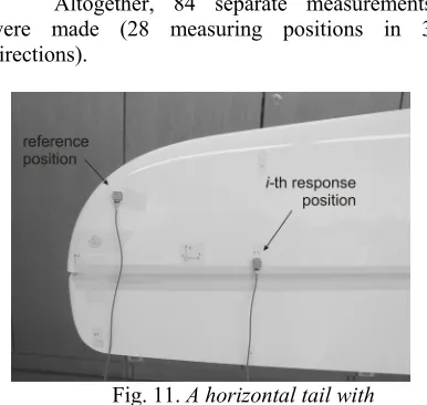
In order to reduce the experimental complexity and the number of nonlinearities in the system, the tail was supported free-free. Twenty-eight measuring positions were defined on the tail’s surface, as shown in Fig.10.
Altogether, 28 local coordinate systems were defined in such a way that the z axis was normal to the surface and the x axis followed obvious lines in the tail geometry. As a reference, measurement position 11 was chosen (Figs. 10 and 11), oriented in the local direction z. Table 1. MAC(ΦX, ΦA)matrix
Mode 1 2 3 4 5 6 7 8 9
0.9994 0.0001 0.0815 0.0000 0.0765 0.0001 0.0742 0.0001 0.0553 0.0001 0.9996 0.0000 0.0750 0.0000 0.0751 0.0000 0.0708 0.0000 0.0695 0.0001 0.9995 0.0001 0.0751 0.0000 0.0751 0.0000 0.0588 0.0002 0.0700 0.0000 0.9992 0.0000 0.0762 0.0002 0.0758 0.0000 0.0672 0.0000 0.0709 0.0000 0.9995 0.0001 0.0781 0.0000 0.0668 0.0001 0.0701 0.0000 0.0728 0.0001 0.9992 0.0002 0.0839 0.0000 0.0683 0.0000 0.0706 0.0000 0.0757 0.0001 0.9997 0.0001 0.0885 0.0001 0.0692 0.0001 0.0716 0.0002 0.0807 0.0000 0.9992 0.0000
MAC
(ΦX, ΦA)
0.0554 0.0000 0.0582 0.0000 0.0639 0.0000 0.0851 0.0001 0.9997 Table 2. Beam’s natural frequencies and damping ratios
i 1. 2. 3. 4. 5. 6. 7. 8. 9.
fi [Hz] 26.08 71.60 140.63 232.73 347.88 486.25 647.93 832.62 1040.7
ζi .104 3.567 1.895 20.649 1.311 1.035 0.9178 1.502 0.8018 0.5266
Fig. 8. Modal assurance criterion matrix
Fig. 9. Horizontal tail in isometric view
In each measurement two signals were sampled:
- the acceleration at the reference position in the reference direction,
- the acceleration at the response position in one of the defined local axes.
Altogether, 84 separate measurements were made (28 measuring positions in 3 directions).
Fig. 11. A horizontal tail with accelerometers placed at the reference position
(left) and at the i-th response position (right)
In order to transform the identified displacements from the local to the global coordinate system, special software was developed by the authors, to which an arbitrary geometry can be imported. The geometrical characteristics are imported into the software in the form of a finite-element-method mesh that consists of volume elements. The user defines the positions and the orientations of the local coordinate systems and the corresponding identified displacements of the single mode shape. The software generates a script which can be run in ANSYS and gives a reconstructed mode shape in the form of a static problem solution.
The identified natural frequencies and the damping ratios are shown in Table 2, and the experimentally reconstructed normalized mode shapes are shown in Fig. 12.
Table 2. Horizontal tail’s natural frequencies and damping ratios
i fi [Hz] ζi .104
1. 22.8 63.17 2. 43.4 83.89 3. 75.5 141.8
a) First mode shape
b) Second mode shape
c) Third mode shape
Fig. 12. Reconstructed normalized horizontal tail’s mode shapes
3 DISCUSSION
From the validation experiment, which served as an ideal, real system, it is obvious that the identified mode shapes agree with theoretical mode shapes to a high degree, although some changes in mass matrix occured due to the displacement of a response accelerometer. With the simple beam experiment the applicability of the continuous wavelet transform to determine the modal parameters is confirmed. A measurement approach with the introduction of a reference accelerometer was shown to be suitable.
According to the experiment realization and the results, performed and obtained in Section 2.2, the presented approach provides a simple and feasible method for an experimental determination of the modal parameters. Although a mechanical system, such as a horizontal tail, is not an ideal system without nonlinearities, the extraction of its modal parameters with a CWT was shown to be a robust and effective method.
4 CONCLUSIONS
continuous wavelet transformation of system impulse response was presented. The computation error due to the finite Taylor series was indicated and its influence on the mode-shape reconstruction was shown. Steel beam mode shapes were reconstructed and compared to the theoretical mode shapes. The spatial mode shapes of a free-free supported horizontal tail of an ultralight aircraft were reconstructed.
A comparison among the theoretical and experimental mode shapes of the beam confirmed the suitability of the proposed method for mode-shape reconstruction. The main contribution of this paper is an enhancement of known methods for EMA using a CWT for one-dimensional cases with a new method for the reconstruction of spatial mode shapes for an arbitrary geometry. In this case it is a horizontal tail. The experimental results can be used for the validation of the numerical model.
5 ACKNOWLEDGEMENT
The authors would like to thank Pipistrel d.o.o. for providing the horizontal tail of the ultralight aircraft.
6 REFERENCES
[1] Maia, N.M.M., Silva, J.M.M. Theoretical and experimental modal analysis, Research Studies Press, Somerset, 1997.
[2] Ewins, D.J. Modal Testing: Theory and Practice, Research Studies Press, Lechtworth, 1986.
[3] Čermelj, P., Boltežar, M. An indirect approach to investigating the dynamics of a structure containing ball bearings, Journal of Sound and Vibration, 2004, vol. 276, no. 1/2, p. 401-417.
[4] Čermelj, P., Boltežar, M. Modelling localised nonlinearities using the harmonic nonlinear super model, Journal of Sound and Vibration, 2006, vol. 298, no. 4/5, p. 1099-1112.
[5] Boltežar, M., Čermelj, P. Dynamics of complex structures - valid modeling of industrial products, In: Korelc, J., Zupan, D. (Eds.): Kuhelj's days 2007, Snovik, p. 17-24, 2007 (in Slovenian).
[6] Mallat, S. A wavelet tour of signal processing, Academic Press, 1999, 2nd
edition.
[7] Staszewski, W.J. Identification of damping in mdof systems using time-scale decomposition, Journal of Sound and Vibration, 1997, vol. 203, p. 283-305.
[8] Slavič, J., Simonovski, I., Boltežar, M. Damping identification using continuous wavelet transform: application to real data, Journal of Sound and Vibration, 2003, vol. 262, p. 291-307.
[9] Slavič, J., Boltežar, M. Enhanced identification of damping using continuous wavelet transform, Strojniški vestnik - Journal of Mechanical Engineering, 2002, vol. 48, no. 11, p. 621-631.
[10] Boltežar, M., Slavič, J. Enhancements to the continuous wavelet transform for damping identifications on short signals, Mechanical systems and signal processing, 2004, vol. 18, no. 5, p. 1065-1076.
[11] Simonovski, I., Boltežar, M. The norms and variances of the gabor, morlet and general harmonic wavelet functions, Journal of Sound and Vibration, 2003, vol. 264, p. 545-557.
[12] Boltežar, M., Simonovski, I., Furlan, M. Fault detection in DC electro motors using the continuous wavelet transform, Meccanica, 2003, vol. 38, no. 2, p. 251-264. [13] Le, T.P., Argoul, P. Continuous wavelet
transform for modal identification using free decay response, Journal of Sound and Vibration, 2004, vol. 277, p. 73-100.
[14] Lardies, J., Gouttebroze, S. Identification of modal parameters using free decay response, International Journal of Mechanical Sciences, 2002, vol. 44, p. 2263-2283.
[15] Huang, C.S., Su, W.C. Identification of modal parameters of a time invariant linear system by continuous wavelet transform, Mechanical Systems and Signal Processing, 2006, vol. 21, p. 1642-1664.
[16] Česnik, M., Slavič, J., Boltežar, M. Modal parameter identification using continuous wavelet transform, In: Boltežar, M., Slavič, J. (Eds.): Kuhelj's days 2008, Cerklje na Gorenjskem, p. 41-48, 2008.