Location as a Poverty Trap
Purti Sharma∗ Niloo Kumari∗∗
Abstract:
In this paper, we ask “Can proximity to towns reduces poverty in rural areas?” For this study we have mapped all the villages in Orissa. The study is based on small area poverty estimation methodology as well as the secondary data covering 47,395 villages and 109 towns. Our main findings are (i) there is a relationship between the distance to nearest town and rural poverty and (ii) poverty levels in rural areas differ according to the type of towns near them and (iii) The combined effect of distance to nearest town and class of town has an U-shape. The study also has various interesting policy as well as regulatory implications.
Keywords: distance, poverty, nearest town JEL Classification: R11, R12, I132
Introduction
There is no doubt that India by and large still lives in our villages. But the development process of the past six decades has made a significant difference. The total population of the country has increased from 361 million in 1951 to 1027 million in 2001, whereas urban population has increased from 62 million to 285 million, rural population has increased from 300 million to 740 millions. This means, while rural population has increased by a factor 2.5, the same for urban is 4.5! According to Census 2001 data, 27.7 percent of our population now lives in urban India.
∗ ([email protected]) India Development Foundation ∗∗([email protected]) India Development Foundation
Annual population growth rate in India -2 -1 0 1 2 3 4 5 1950 -55 1955 -60 1960 -65 19 65-70 1970 -75 1975 -80 1980 -85 1985 -90 1990 -95 19 95-00 2000 -05 2005 -10 2010 -15 2015 -20 2020 -25 2025 -30 2030 -35 2035 -40 20 40-45 2045 -50
Urban annual population grow th rate Rural annual population grow th rate
Source: Department of Economic and Social Affairs of the United Nations Secretariat, World Urbanization Prospects, 2009
Graph: 1 Annual Population Growth Rate in India
As per UN estimates from The World Urbanization Prospects, 2009, the compound annual growth rate of urban population in India will be 2.4 percent every five year from 2010 to 2030. By this rate of growth, India’s urban population is estimated to reach 590 million by 2030. The five-yearly annual growth rate of urban population has been more than that of the rural population due to the rapid urbanisation process. The gap between the urban and rural population was expected to increase at a rapid pace from 2000-05 onward which we can see from graph 1. And this pace is expected to continue if India remains on its path of high growth.
This rapid growth is a result of two factors i.e. natural growth rate of the population and migration from rural to urban areas. The urban and the rural economy are inter-dependent. The dependence of villages on the urban area is quite visible in terms of migration, employment opportunity
and infrastructure (Gangopadhyay, 2009) 1.In this paper we are limiting
our scope of study by only looking into rural dependence on urban area.
In India migration has taken place from villages to towns and cities in
search of better income opportunities1. ‘Poverty-push’ and
‘prosperity-pull’ factors coupled with the expectations that urban area offers, diverse opportunities for employment and better living conditions in term of infrastructure, housing, water, health facilities etc are the major cause for this. We observe that in rural area the poor’s are less organized as compared to the urban poor (European Commission, 2008).This is because rural population is more geographically dispersed and inhabiting remote areas. This makes it much more costly to deliver social services to poor people in the dispersed areas. Therefore, it is natural to ask the question: What would be an effective targeting? Should it be developing models that can reach remote areas better or can one count on spillover effects to take care of poverty in the remote areas?
Although it is intuitive that the level of poverty is likely to be significantly high for those living in remote areas, but so far there has been relatively little quantitative evidence to substantiate this. More recent is New Economic Geography models, which emphasised on distance and regional economics in general. But there have not been any studies that have empirically assessed the nexus between poverty in rural areas and
their geographic proximity to urban area in India. European Commission
report (2008) described four categories of problems of rural areas i.e. demography, remoteness, education and labor market which may interact and generate “vicious circles” of poverty in rural areas. The report also describes that the differences between rural and urban areas may be the result of a decentralised decision-making process which gives regional and local authorities policy discretion and therefore permits regional differences in funding. They have also found that it is difficult and costly to deliver social assistance to poor people in areas characterized by dispersed population and problems of remoteness. Similarly, Monica Fisher (2004) tried to study whether living in rural area is associated with a higher risk of poverty in United States. This study found that non metro households have a 19 percent higher probability of being poor compared with metro household. The proximity of any rural area to a town lowers transportation costs, lowers costs of obtaining information about demand and supply conditions, reduces service delivery cost and may foster knowledge spillovers between urban and rural. But there are different tiers
1
of town depending on their population and hence they would differ in their infrastructural facilities. So there would be a difference in the spillover effects of different tiers of town on their nearby rural areas. Nord (1998) suggests that the out-migration is a positive force for those who move on to better opportunities elsewhere, but it can also concentrate poverty because those who remain behind when a community falls into economic decline are those with fewer opportunities.
The exponential population shifts from rural to urban area leads to a rapid urbanization. But regions or areas have evolved differently due to spatial externalities and agglomeration effects. This disparity in growth lead to the question; how and which class of the towns should be targeted
for development?1 Should the government investment be top-down
planning or bottom- up planning or leave it on organic growth of the towns? Secondly, out of these strategies which will lead to stimulate more economic growth? We will answer these questions in the last section of our study. In different countries for example Brazil and Philippines, few towns are selected and a huge amount of money is poured into them in the form of infrastructure investment. The basic idea behind that is to improve accessibility and to benefit surrounding areas with the trickle down effects. The government of India also initiated centrally-sponsored Scheme of Integrated Development of Small and Medium Towns (IDSMT) during the Sixth five year plan (which continued in the Seventh and Eighth Plans also). Its main objective was to slow down migration from rural areas and smaller towns to large cities by the development of selected small and medium towns which are capable of generating economic growth and employment. However, since the inception of the scheme only about 40 percent of the towns could be covered out of more than 4600 eligible towns.Most of the urban local bodies were not in a position to avail loan
from financial institutions to partly finance the IDSMT scheme 2 .There
were other implementation issue also like non-availability and non-release of matched state share by the state government within the specified time, non-submission of utilisation certificates in time by the States etc. Taking note of IDSMT scheme’s shortcomings, the Central government has
1 The census 2001 has divided urban towns into six classes/Tiers based on population. The towns with
population of 100,000 and above are classified as Class I or tier I cities, population between 99,999 to 50,000 as Class II or tier II cities, population between 49,999 to 20,000 as Class III or tier III cities, population between 19,999 to 10,000 as Class IV or tier IV cities, population between 9,999 to 5,000 as Class V or tier V cities and population less than 5,000 as Class VI or tier VI cities.
2 According to the 74th Amendment Act, 1992, granted constitutional status to a third-tier of government in the
recently developed two strategies: First, the Jawaharlal Nehru National Urban Renewal Mission has been sanctioned in year 2005 to provide extensive financial support to about 60 cities for up-gradation and improvement of infrastructure in a planned and integrated manner. These cities comprise the State capitals, cities with one million plus population and some selected cities of religious, tourist, cultural and heritage importance. It is expected that these cities will have a demonstration effect on others. The second approach was to identify the need of other cities and towns, which are not included in the Mission, is sought to be addressed through an assistance of scheme known as “Urban Infrastructure Development Scheme for Small and Medium Towns (UIDSSMT)”. The government’s objective with these two approaches is to bring in those improvements that will enable the town-level institutions to become financially strong and viable. This will also help government’s development related programmes, which is working towards removal of poverty to become more bankable.
India (46.4 percent BPL population) and also because it has the highest poverty deviation within districts in rural areas (Gangopadhyay et al (2010; 2011). The district wise poverty estimates for the given states are calculated using small area estimation methodology.
The rest of the paper is organised as follows. Section II presents the data description and their sources. Section III will outline the empirical models used to test the hypothesis and its results. Finally, in section IV we provide suggestions and conclude.
II. Data Description and their Sources
•Census Data
We have used Census, 2001 household dataset on general & socio-cultural characteristics. The basic information collected regarding general and socio-cultural characteristics are on religion, mother tongue, languages known, literacy and educational status, characteristics of workers and non-workers, migration characteristics and fertility particulars etc. It also collects information on the basic amenities available at the village and town level. For the present study we have used the Census 2001 household data as well amenities data.
•NSS Data
In the present study, we have used NSS 61st Round Consumer Expenditure survey held during the year 2004-05. It was conducted on large sample basis and it was the seventh quinquennial survey on the subject. The survey provides information on monthly per capita consumption expenditure by 32 broad groups (14 food groups and 18 non-food groups) of items of consumption. The per capita consumption estimates are provided separately for rural and urban sectors of each State and Union Territory. The poverty estimates of the year 2004-05 for the Orissa is based on the consumption expenditure survey of the NSSO, which has a sample size of around 5023 households.
•Poverty estimates
experimented with, for identifying specific local government levels having the worst human development outcomes.
The basic methodology for small area estimation for poverty maps was developed by Elbers, et al. (2002; 2003). The approach involves the estimation of a household consumption model from survey data that is then applied to individual households in the census data to predict their consumption levels. In principle, then, if these predictions of individual household consumption levels have been correctly done then one can aggregate them to any desired level such as blocks and districts by sectors (i.e. rural or urban) , to get poverty estimates at that level. Since of course, the actual method is a bit more involved and one can look at Gangopadhyay et al (2010; 2011) for a more complete description.
There are three distinct parts to the exercise. First, a comparison of common variables across the household survey and the population census is undertaken. The idea here is to identify variables at the household level that are defined in the same way in both the household survey and the census. It is important that this common subset of variables be defined in exactly the same way across the two data sources. The common variables in these two data i.e. the census and survey are chosen on basis of similar distributional properties. The second part of the analysis involves the econometric estimation of models of consumption using the set of household-level and community variables. Extensive exploration of alternative model specifications is undertaken so as to identify those which can most reliably and successfully serve as foundation for predicting welfare outcomes in the census.
Successful completion of the second-stage analysis permits one to take the parameter estimates to the final part of the exercise. This stage is associated with the imputation of the poverty indicators into the census data at the household level and the estimation of summary measures of poverty, at various levels of spatial disaggregation. Statistical precision of the poverty estimates is also gauged in this stage.
The estimation procedure is well spelt out in Elbers et al.(2001;2002). The methodology proposed has two stages. Firstly, a model of log per
capita consumption expenditure ( ) is estimated in the survey data:
Where is the vector of explanatory variables for the household in the
vector of location specific variables with being the associated vector of
coefficients, and is the regression disturbances due to the discrepancy
between the predicted household consumption and the actual value. This disturbance term is decomposed into two independent components:
Where,
is a cluster-specific effect and is a household-specific effect. This
error structure allows for both a location effect – common to all households in the same area – and heteroskedasticity in the household-specific errors. All parameters regarding the regression coefficients
and distributions of the disturbance terms are estimated by Feasible Generalized Least Square (FGLS).
In the second part of the analysis, poverty estimates and their standard errors are computed. There are two sources of errors involved in the
estimation process: errors in the estimated regression coefficients and
the disturbance terms, both of which affect poverty estimates and their levels of accuracy. ELL propose a way to properly calculate poverty estimates as well as measure their standard errors while taking into account these sources of bias. A simulated value of expenditure for each census household is calculated with predicted log expenditures
and random draws from the estimated distributions of the disturbance
terms, and .These simulations are repeated 100 times. For any given
location (such as a district or a village), the mean across the 100 simulations of a poverty statistic provides a point estimate of the statistic, and the standard deviation provides an estimate of the standard error.
Methodology
After obtaining the poverty estimates we merged the rural and urban data on the basis of distance of nearest town from a village. Table 1 presents descriptive statistics of number of villages nearest to the towns by town class. Among all town classes, highest percentage of villages falls in the Tier III (i.e. 36 percent) followed by Tier IV (i.e. 26 percent) category. We found that for some villages of Orissa, the nearest town was located in the bordering state i.e. Andhra Pradesh. So in this study we have taken its impact into consideration as well.
VI category. Table 3 presents the spatial distribution of villages by distance classes. Distance to nearest town for a given village is the number of kilometres between village ‘i’ to the closest urban town. It is quite possible for a village to have better access to a town, which might not the nearest town in term of distance. But the present study is restricted to distance to the nearest towns only. In order to evaluate the impact of distance, we divided the distance into six categories: i) between 1 km and less than 10 kms, ii) between 10 kms and less than 20 kms, iii) between 20 kms and less than 30 kms, iv) between 30 kms and less than 40 kms, v) between 40 kms and less than 50 kms, vi) between 50 and more. We have converted variable ‘distance to nearest town’ from continuous to category variable. We have done this to eliminate the outliers.
One of the shortcomings of our study is that closeness to a town does not imply easy accessibility to that town. For example in coastal areas, desert or islands time taken to travel few kilometres can take longer so the impact of distances measured in kilometres would not have similar impact as it would have been in villages well connected to the towns. We have chosen Orissa for our study which has plane land and hence such issues can be neglected.
III. Empirical specifications
In India, the consumption expenditure is used as proxy for income to predict poverty. The poverty estimates is published by the Planning Commission. It counts the below poverty line population using monthly per capita consumption expenditure data from the NSSO. In the present study, we have used poverty line published by the Planning Commission for the year 2004-05. The NSS 61st round consumption expenditure data is not representative at the lower levels of disaggregation, so we have use OLS model for income prediction using Small area estimation methodology which had estimated head count ratio (HCR) or also known as poverty ratio (details mentioned in data description section).
The percentage of population below poverty line published by the Planning Commission for the state of Orissa is 46.4 percent in year
2004-05 based on UPR-Consumption1. The reported urban poverty is 44.3 and
the rural poverty is 46.8 percent. In the present paper have considered 105 towns in Orissa and 4 towns from Andhra Pradesh and divided them into
1 URP consumption = Uniform Recall Period consumption in which the consumer expenditure data for all the
six Tiers based on their population size. The towns from Andhra Pradesh are considered because for some villages in the bordering areas of Orissa had those towns nearest to them. Table 2 shows that the Tier IV has highest percentage of towns i.e. 37 percent out of the total number of towns. And the least number of towns are in the VI Tier. We had data available for 47395 villages in Orissa. Out of the total villages, 14.12 percent lies within 0-10 km, 22.75 percent lies within 11-20 km, 20.32 percent within 21-30 km, 15.59 percent lies within 31-40 km, 10.06 percent lies within 41-50 km and 17.16 percent lies more than 51 km away from the town.
The graph 2 below shows the distribution of the head count ratio across the villages in Orissa. The x-axis represents the head count ratios divided into ten below poverty line (BPL) classes. Similarly, the y-axis represents the percentage of villages falling into each BPL class. The percentage scales the height of the bars so that the sum of their height equals 1. From the graph we observe that 15 percent of villages have BPL population between 0 to 10 ratios. The highest proportion of villages’ i.e.28 percent has 90 to 100 ratio of population below poverty line. The overall estimated rural poverty for Orissa is around 44.9 percent using the poverty line given by Planning Commission for the year 2004-05.
0
10
20
30
Pe
rc
e
n
ta
g
e
o
f
Vi
lla
g
e
s
0 .2 .4 .6 .8 1
Head Count Ratio
Graph for Head Count Ratio
In this section, we present two empirical models. One assesses the effect of distance to nearest town on rural poverty and other shows the effect of nearest class of town on the rural poverty.
First, to estimate the effect of distance to nearest town on rural poverty the OLS model was used. The basic specification, which was estimated at the level of village, is given below:
(1)
where represents rural head count ratio, is a measure
of distance of nearest town from the village, is error term where
i=(1,2,3…n). The specification is given at the village level because it is the
lowest level of disaggregation at which poverty estimates were calculated for the state of Orissa. The regression results are presented in Table 4 (model 1). All the variables are significant at 1 percent level of significance.
In table 4, (Model 1) we have used distance to nearest town from the village as dummy variable. Here the result shows that distance has a negative impact on poverty. The highest level of poverty decrease is for those rural areas which are between 1 km and less than 10 km from the urban area as compared to those who are away more than 50 kms. The lowest level of poverty decreases for the category between 40 kms and 50 kms if we take distance to nearest town more than 50 kms as base. We have chosen the base to avoid falling in the dummy variable trap.
is chosen as a base to make the interpretation of the result easily
comparable with the other dummies..The results in the table 4 show that as
compared to , being closer to a town would have a higher
Graph 3: Percentage of Rural Poor by Distance to Town
The graph 3 clearly shows that with every successive increase in distance from the town, the rural poverty increases. It appears that there is a high degree of association between poverty and infrastructure also (Editor’s desk, 2009). So we also expect to find that the poverty is lower and public service availability is higher in towns than in the remote areas. And availability of good quality infrastructure is an essential prerequisite for the growth. This could be because of government’s policy biasness towards urban or near urban area while allocating resource. From the above equation 1 we found a clear pattern that the rural poverty deceases due to the urban proximity as well as urban spillovers. We will now try and find out how poverty reduces when each distance class is individually regressed on poverty. This is done using the equation given below.
(2)
where i represents villages in each distance category i.e. 6693, 10781,
9631, 7388, 4768 and 8134 villages in distance class 1,2,3,4,5 and 6 respectively. Here k= (1, 2, 3, 4, 5, 6) represents the different category of distance class.
the poverty reduction is highest for the category of distance between 1 km and less than 10 kms followed by category of the distance class between 10 kms and less than 20 kms. When we regress distance class between 30 kms and less than 40 kms on poverty estimates we find a positive impact on poverty. The villages those are more than 50 kms away from the closest town reflects the highest level of poverty increase compared to other categories. Here all the explanatory variables are significant at 1 percent level of significance.
The causes of rural poverty are complex and multidimensional. They involve things like culture, climate, gender, access to markets, public policy etc. Likewise, the rural poor are quite diverse both in the terms of problems they face and available solutions to these problems. Broad economic stability, competitive markets, and public investment in physical and social infrastructure are widely recognized as important requirements for achieving sustained economic growth and a reduction in rural poverty. We saw from the above result that if a village is in close proximity to a town they are better off as compared to those villages in remote areas. This could be mainly because they would have more employment opportunities and an easy market access. There would also be spillover effects on these villages from the nearby towns.
dummy variables in our regression to find what is the effect of different classes of town on the rural poverty (refer Table 5). Here we have not used any filters other than population to explain the class of cities. There might be cities which are administrative hub or market hub which would have different impact on poverty. For example, the villages which are closer to
the town along with presence of ‘mandi’ would have a different impact on
poverty as compared to same tier of town which do not have a ‘mandi’1.
Since mandies are also not comparable (some might be for perishable
goods where as others might be for non perishable good) so we have not taken them into consideration in this study.
(3)
Where, t is categories of town classes. We do not see a clear cut pattern of
the impact of different classes of town on rural poverty from the regression result. The result is given in table 5, in model 8 column. It shows that if rural regions are closer to tier I, tier III and tier IV the town has negative coeffient i.e. poverty falls. Only tier I town is significantly affecting poverty, rest of the variables are insignificant at 5 percent level of significant. Here the types of towns are taken as dummy variable. We have take tier VI as our base for the regression models.
(4)
where ‘i’ represents number of towns in Orissa and Andhra Pradesh, ‘t’ is
categories of town classes2. In table 5, (Model 9 to model 14) we have
tried to find out the impact of different class of towns on the rural poverty individually. Though all the tiers are significantly impacting poverty but we do not find any clear cut pattern when regressed individually. We expected that villages closer to bigger towns would have lower poverty as compared to those nearer to the smaller towns, since the classes of towns
are based on the urban hierarchy3. Table 5 show that tier I and III towns
has a negative impact on rural poverty where as other tiers of town has a positive impact on poverty.
(5)
1
Business / Commerce market in India
2
Some of the nearest villages are in the bordering areas of Orissa that had nearest towns in Andhra Pradesh so we included those towns in our study as well.
3 Towns are divided into different tiers based on their population. Tier I having the highest category of
From the above regression result we know that both distance and class of the town matters. However there is no uniform impact of town hierarchy on poverty rate. In order to estimate the combine effect of distance and
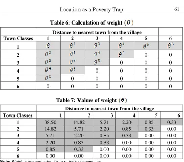
class of towns on poverty rates we created the weight (wt) variable. It has
two properties 1) the values add up to one 2) values are non-increasing (refer Table 6). The purpose of creating this weight matrix was to find the combined effect of distance to town and town classes. We would also like to measure the maximum spillover impact of town class and distance on the poverty. We want to answer the question we posed at the beginning of this paper i.e if the policy maker has an amount X earmarked for eradicating rural poverty. It can either spend the entire money for direct poverty interventions in the rural areas or can spend only a part of it there. Now the crucial question is how to utilize the remainder. Should it target large metros or smaller towns? The answer to this question would depend upon the possible spillovers effect of a large metro or a relatively small town would have on its neighbourhood rural areas.
Now if the policy makers choose the second approach, we would try and answer how to utilize the remainder money. We have six categories of distance to town and tiers of town. The matrix is created such that different weights are given to different combination of distance classes and tier of town. The weights are non- increasing meaning combination of tier I town and disclass 0-10 would have a higher weight than same tier and disclass 11-20 and so on. Similarly combination of disclass 0-10 and tier I would have a higher weight as compared to same disclass and ties II and so on. This matrix also adds up to 1. Table 7 below shows the weight matrix that we have used.
In equation 6 represent weights, represents square of weight
we have calculated the minimum point till where the weights would have a negative impact on poverty. It comes to be 22.68
Graph 4: Relationship between poverty and weights
The graph 4 shows that the relationship between the poverty and weights. The y-axis represents the Head count ratios (HCR) and x-axis represents weights. The weights are the combined effect of distance to nearest town and class of towns. The higher weights are given to bigger towns and closer rural areas in terms of distance. We find an U-shaped curve. The above graph shows that the poverty reduces till a point, and after that it starts increasing. The lowest point of the U- shape curve is 22.68. This
value is between two combinations i.e disclass 2 & Tier 1 cities and
III and VI cities have a much weaker position than the Tier I and II cities. However, due to massive urbanisation Tier I and II cities have disadvantages such as high property prices, high density of population, traffic congestion, crime and environmental pollution etc. On the other hand, the Tier III and IV cities appear better in managing and controlling these issues. So we have reasons to assume that Tier III and IV cities have specific potentials to compete with Tier I and II cities in terms of establishing new firms and industries. We know that the Tier III and IV cities are less equipped in terms of critical mass and institutional & organizing capacity. But they offer assets and resources which are not available in abundance in Tier I and II cities. So, if the government invests Tier III and IV cities especially in infrastructure, then it will attract more investment from private sector as well.
IV. Summary and Conclusion
Annexure:
Table 1: Number of Village Nearest to the Towns by Town Class
Town classes Villages
Tier I 6394
Tier II 9863
Tier III 17211
Tier IV 12949
Tier V 954
Tier VI 24
Total number of villages 47395
Note: The study has not considered those villages were the distance to nearest town is reported to be zero. This is because name of the town was missing in the rural dataset. As a result we could not merge rural and urban datasets.
Source: Census 2001, India
Table 2: Number of Towns by Town Classes
Town classes Towns
Tier I 8
Tier II 15
Tier III 36
Tier IV 41
Tier V 8
Tier VI 1
Total number of town 109
Source: Census 2001, India
Table 3: Number of Villages by Distance Classes
Distance to town Villages
dist_town_0_10 6693
dist_town_11_20 10781
dist_town_21_30 9631
dist_town_31_40 7388
dist_town_41_50 4768
dist_town_51_above 8134
Total number of villages 47395
Table 6: Calculation of weight
Distance to nearest town from the village
Town Classes 1 2 3 4 5 6
1
2 0 0
3 0 0 0
4 0 0 0 0
5 0 0 0 0 0
6 0 0 0 0 0 0
Table 7: Values of weight
Distance to nearest town from the village
Town Classes 1 2 3 4 5 6
1 38.50 14.82 5.71 2.20 0.85 0.33
2 14.82 5.71 2.20 0.85 0.33 0.00
3 5.71 2.20 0.85 0.33 0.00 0.00
4 2.20 0.85 0.33 0.00 0.00 0.00
5 0.85 0.33 0.00 0.00 0.00 0.00
6 0.00 0.00 0.00 0.00 0.00 0.00
Note: Weights are converted from ratios to percentages.
Appendices
From the non-linear equation given below we know that the weight square (i.e. vector of distance to nearest town and class of town) has an inverted U-shape. Hence there would be a value of the weight where the poverty reduction would be optimal after which poverty would start increasing.
(7)
Where, and represent weight and square of weights. In order to find
out the optimal point in the weight matrix (refer to Table 6) we will
differentiate the above equation. To find the optimal value of
which is 22.68 and to find the minimum value the second order
Refrences:
1- Catin M, 1995, “Economies d`agglomeration, Revue d`Economie Ragionale et Urbaine, 4, pp.1-20.
2- European Commission Report, 2008. “Report on Poverty and Social Exclusion in Rural Areas,” Directorate-General for Employment, Social Affairs and Equal Opportunities.
3- Fisher Monica, 2004. “On the empirical findings of a higher risk of poverty in rural areas: Is rural residence endogenous to poverty?” RPRC Working Paper No. 04-09, Rural Poverty Research Centre.
4- From the Editor’s Desk, 2009, Journal of Infrastructure Development, Volume
I
5- Gangopadhyay, Shubhashis 2009 , “How can Technology Facilitate financial
Inclusion in India? A Discussion Paper”, Review of Market Integration, 1(2):
223-256.
6- Gangopadhyay Shubhashis,Ghosh Namrata and Sharma Purti, 2010, report on “Generating Poverty Maps for India” , submitted to Planning Commission
7- Gangopadhyay Shubhashis,Ghosh Namrata, Sharma Purti and Kumari Niloo (2011), report on “Generating Poverty Estimates Using New Poverty Lines”, submitted to Planning Commission
8- Gibson John, Deng Xiangzheng, Gibson Geua Boe, Rozelle Scott and Huang Jikun, 2008. “Which Households Are Most Distant from Health Centers in Rural China? Evidence from a GIS Network Analysis,”
9- Partridge Mark and RickmanDan S., 2008. “Distance from Urban
Agglomeration Economies andRuralPoverty,” Journal of Regional Science
48(20), 285-310.
10- Quigley JM, 1998, Urban Diversity and Economic Growth, Journal of Economic Perspective, 12, pp.127-138.
11- Nord M., 1998. “Poor people on the move: county to county migration and
the spatial concentration of poverty,” Journal of Regional Science 38(2),
329-351.
12- Ruspaingha Anil, Goetz, 2007. “Social and political forces as determinants of poverty: A spatial analysis,” The Journal of Socio-Economics 36, 650–671. 13- Weber Bruce, Jensen Leif, Miller Kathleen, Mosley Jane and Fisher Monica, 2005. “A Critical Review of Rural Poverty Literature: Is There Truly a Rural Effect?” Discussion Paper no. 1309-05, Institute for Research on Poverty.
14- William R. Easterly and Ross Eric Levine, 1997. “Africa’s growth tragedy: