Focal Stack Image Fusion Using Image Volume Reconstruction

2016 International Conference on Artificial Intelligence and Computer Science (AICS 2016) ISBN: 978-1-60595-411-0

Focal Stack Image Fusion Using Image Volume Reconstruction

Tao ZENG

_{, Chang-Yu DIAO}

_{and Zhuo-Hao LIU}

1_{College of Computer Science and Technology, Zhengjiang University, HangZhou, China}

2_{The Cultural Heritage Institute, Zhengjiang University, HangZhou, China}

E-mail:a _{[email protected],}b _{[email protected],}c _{[email protected]}

Keywords: Focal stack images, Focus measure, Non-blind deconvolution.

Abstract. Traditional camera can’t take photos with large depth of field (DOF) because of the lens limits. The region out of DOF often gets blurred due to narrow width of depth. Focal stack photography take a set of (three and above) pictures viewing the same scene with different focus point and fusion the pictures as one using computational algorithms in order to have all-in-focus photos. Some state-of-art focal stack algorithms seek the best-in-focus point among these stack photos and collect them into a new all-in-focus image. This method is derived from the assumption that at least one photo in the stack has the clear vision of the point of the scene. But what if none of these points are in focus because unfortunately focus point falls out of the object of the scene? Focal stack images not only provide us several pictures independently but also partial information about how the object is imaging at a certain depth. With this information, we seek a space called ‘image volume’ to search the best in-focus depth beyond the two dimensional images to avoid the failure mentioned above. We work through the whole scene space and find the accurate depth of every point in the scene. We experiment some pictures with focal stack example and show better results than traditional methods.

Introdution

Traditional photography requires camera parameters to be strictly precise when taking a picture. Unfortunately, image blur due to defocusing or camera shaking happens occasionally. We often want to take pictures with wide DOF (depth of field) of the scene, but sometimes we can’t get satisfactory DOF because of the lens limits of the camera.

Scene depth outside the DOF is called defocused or defocus blurred and information like edges and corners are lost due to defocus blur. We can extend the DOF by carefully choosing the camera parameters in some extent, such as switching to a smaller diameter. However diffraction may happen when you set the diameter too small and causing the degradation of the image. This could be critical when you want to get images with wide DOF and low degradation. As a result, there has been a trade-off between degradation and extended DOF.

Extending the DOF of a scene and generating an all-in-focus image has been a popular and fundamental research problem in computer vision [1,2,3,4] and optics[5]. This could be critical for various low-level vision algorithms relying on pixel level image information, e.g. segmentation. Additionally, partially focused images are not visually pleasing which are often discarded.

Currently available consumer products that supporting post-capture refocusing, flexible control and extension of depth of field such as light field cameras require extensive modification of the sensor and hardware, meanwhile light field cameras currently achieve only low image resolution. Depth and light field cameras requires post-processing algorithms aim at capturing high-dimensional visual information in a scene, this requires large amount of memory space and cpu capacity.

In contrast, we propose a simple solution by capturing high-resolution focal stack images using a conventional camera, thus reducing the requirement on photographic equipment.

location[2]. A set of images can be captured with consecutive depth-of-field(DOF), hence small amount of blur occurs in every image, but we can jointly recover the latent image. In this paper, we propose a multi-image deblurring system that combines two existing techniques: blur kernel estimation and non-blind image deconvolution. A series of images is captured while the camera lens is sweeping through the camera optical axis and the data is recorded simultaneously. By measuring camera settings(ISO, focal length and aperture of the lens) and align the scene as accurately as we can, we improve the restoration of the defocus blurred images.

Related Work

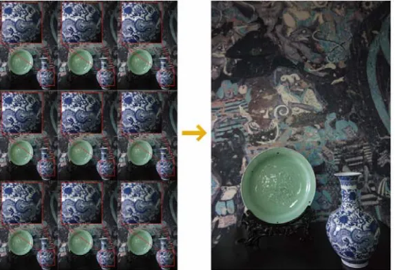
Usually, the slices of a focal stack are combined to create a single AIF image (Figure 1). Hasinoff and Kutulakos [8] analyzed the optimal settings for focus and aperture to minimize the number of required photographs for a given depth range. Levin [9] capture a single image using coded aperture and use calibrated blur kernels to simultaneously obtain depth and an all-in-focus image. There are researches and prototypes and even commercial products demonstrate that light field cameras or plenoptic cameras can extend the DOF of an image and refocusing images after being taken[10,11,12]. But this kind of cameras need special designed microlens and extra memory space compared with conventional cameras. Besides, the resolution of light field cameras is not able to surpass that of conventional digital cameras.

Figure 1. focal stack images(left), all-in-focus image(right).

We often use image gradient or laplacian based measures as focus measure to evaluate how much an image is blurred. Huang and Jing [13] assess focus measures from defocused image blocks and find SML provide better performance than other focus measures. Kumar and Ahuja[14] propose a generative focus measure using convolution to identify the most focused image.

The measure gives a quantitative estimate of how focused an image is in any one of the given focal stack images. But not all the focused pixels lie exactly in the focal stack images we captured, they may exist in between two adjacent images. Nayar and Nakagawa [2] use Garssian distribution to interpolate the computed focus measures to obtain more accurate depth estimates. Thus, the best estimated depth of an object lies between two stack images. Hasinoff, et.al. [8] have also shown that omnifocus image obtained using focal stack usually have a higher signal-to-noise(SNR) ratio as compared to single shot based techniques.

Focal Stack Photography

Focal stack images are pictures taken by different camera settings but with the same scene and the same scale. One kind of focal stack is diameter-variant, fixing the focal length and adjusting the diameter of the camera to different depth of field. Another focal stack is fixing both focal length and diameter bur adjusting the focal point from near to far range of the scene. We choose the latter pattern to constitute the focal stack images. All the DOFs of the stack images constitute the combination of an extended DOF of the scene. After the alignment of the focal stack images, we guarantee the one-to-one correspondence of pixels in the scene within each stack images. Section 3.1 we discuss how to calculate the circle of defocus blur, and we introduce the focus measure we use in section 3.2.

Focal Stack Acquisition

Given a point light source, the intensity spreads wider on frame as farther the distance away from the in-focus frame (Figure 2). The radius of the point spread function can be depicted as [14],

R x, y 1 ; R x, y 1 (1)

in which, D is the diameter of the lens settings, F , F, F denote distances between image and sensor plane. The PSF function is often modeled as a Gaussion distribution,

h x, y _πσ exp _σ (2)

where, σ and c √2[2]. A defocused image f is can be modeled as the following convolution:

f x, y _∞∞ _∞∞l x μ, y ν h μ,ν dμdν. (3) Where l(x,y) is the in-focus image.

Figuer 2. focal stack photography.

In the next section, we will discuss the focus measure and evaluate the blurriness of pixels across the focal stack images.

Focus Measure

Focus measures are discussed a lot in the previous researches, most of them are gradient related and laplacian related[13]. In our method, we just use one of them, Sum-modified-Laplacian(SML), to describe the blurriness of pixels:

SML ∑ ∑ f i, j for f i, j T. (4)

f x, y |2f x, y f x step, y f x step, y |

|2f x, y f x, y step f x, y step |. (5) And T is a discrimination threshold value.

We usually take the maximum value of focus measure to be the best focused location. But there has been some limitation that what if the theoretical best frame lies between two adjacent focal stack images and the maximum value of focus measure can’t be detected in the images now available. There needs to be dealt with the focus measure values.

Depth Estimation and AIF Image Recovery

The focal stack images give us partial information of how an object is imaging at a certain depth. But object points not belong to these certain depth are definitely not in focus. How to evaluate these not-in-stack points becomes a problem. The measure gives a quantitative estimate of how focused an image is in any one of the given focal stack images. But not all the focused pixels lie exactly in the focal stack images we captured, they may exist in between two adjacent images.

As Nayar did in [2], we interpolate the focus measures we computed in every stack image using quadratic curve fitting(Figure 3). d , d , d , d denote the depth location of corresponding focal images, S , S , S , S denote the SML of pixels in corresponding location, and d

denotes the best focused depth position. As long as we find the maximum of the curve, we find the best focused depth at a pixel location. Because of the unimodality of the focus measure[14], there exists one and only best focused depth of a pixel. This best focus depth most likely lies between two adjacent focal stack images. We find the best depth of the pixel location within three-dimensional space (“image volume”) other than in two-dimensional focal stack images in order to spreading the searching widely enough to get closer to the theoretical results of the real world.

Figure 3. quadratic interpolation of focus measure.

As we find the depth of a location, we use Eq. (1) to acquire the circle of blurriness in observed images. After deciding the circle, the blur kernel of PSF function is determined. The non-blind deconvolution RL algorithm alternately accomplishes the defocus procedure of focal stack images.

Experiments and Results

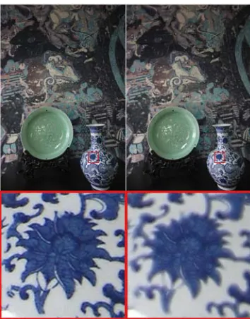
Figure 4. all-in-focus images of “vase” dataset. Left: our method; right: Kumar’s method.

Figure 5. all-in-focus images of “cup” dataset. First line: our method; second line: Kumar’s method.

Then we have quantified the experiment with these above datasets by evaluating some other focus measures of the all-in-focus images discussed in [13]. From Table 1, better or closer focus measure values are observed of our method than the compared.

Table 1. focus measure values of each method.

Dataset Variance

(×103₎

Energy of Gradient(EoG)

(×109₎

Spatial

Frequency(SF) Tenengrad _(×109₎

“vase” Kumar’s 2.1004 3.6938 5.7581 6.8175

Ours 2.0289 5.0779 5.4447 11.932

“cup” Kumar’s 2.6811 4.1703 4.4806 6.7162

Ours 2.5876 4.4174 4.7827 9.6924

Conclusion and Future Work

of PSF model and restore the all-in-focus image with non-blind deconvolution algorithm. Experiment shows good qualities both in visual and quantity observation. Pixel-wised methods like we employ in this paper suffer artifacts like noise and sudden burst of pixel value and we will explore other more effective deconvolution algorithms in the future.

Acknowledgment

This work has been supported by “National Key Technology Support Program (No. 2014BAK16B01)”.

References

[1] E.P. Krotkov. Focusing. Technical Report MS-CIS-86-22, GRASP Lab, University of Pennsylvania, 1986.

[2] S. Nayar and Y. Nakagawa. Shape from Focus. PAMI, pp. 824–831(1994).

[3] A. Krishnan and N. Ahuja. Range estimation from focus using a non-frontal imaging camera, International Journal of Computer Vision, 20(3): pp. 169–185(1996).

[4] N. Xu, K. Tan, H. Arora, and N. Ahuja. Generating omnifocus images using graph cuts and a new focus measure. in Proc. of the 17th International Conference on Pattern Recognition, volume 4, pp. 697 –700(2004).

[5] J. Edward R. Dowski and W.T. Cathey. Extended depth of field through wave-front coding. Applied Optics, pp. 1859–1866(1995).

[6] C. Zhou, D. Miau, and S. Nayar. Focal Sweep Camera for Space-Time Refocusing. Technical report, Department of Computer Science, Columbia University(2012).

[7] M. Subbarao, T. Choi, and A. Nikzad. Focusing techniques. Journal of Optical Engineering, pp. 2824–2836(1993).

[8] S.W. Hasinoff and K.N. Kutulakos. Light-efficient photography. In IEEE Trans. PAMI, pp. 2203–2214(2011).

[9] A. Levin, R. Fergus, F. Durand, and W.T. Freeman. Image and depth from a conventional camera with a coded aperture. In SIGGRAPH, 2007.

[10] E.H. Adelson and J.Y.A. Wang, Single Lens Stereo with a Plenoptic Camera. IEEE Trans. Pattern Anal. Mach. Intell, pp. 99-106(1992).

[11] R. Ng, , M. Bredif, G. Duval, M. Horowitz, P. Hanrahan. Light Field Photography with a Hand-held Plenoptic Camera. Tech Report CTSR 2005-02, Stanford University(2005).

[12] M. Levoy, R. Ng, A. Adams, M. Footer and M. Horowitz, Light field microscopy, in ACM Transactions on Graphics, pp. 924-934(2006).

[13] W. Huang and Z. Jing, Evaluation of focus measures in multi-focus image fusion. Pattern Recognition Letters, 28(4): pp. 493-500(2007).