Estimation of covariance, correlation and precision matrices for high dimensional data

(1)

Estimation of Covariance, Correlation

and Precision Matrices for

High-dimensional Data

Na Huang

Department of Statistics

London School of Economics and Political Science

A thesis submitted for the degree of

Doctor of Philosophy

(2)

(3)

Declaration

I certify that the thesis I have presented for examination for the MPhil/PhD degree of the London School of Economics and Political Science is solely my own work other than where I have clearly indicated that it is the work of others (in which case the extent of any work carried out jointly by me and any other person is clearly identified in it).

The copyright of this thesis rests with the author. Quotation from it is permitted, provided that full acknowledgement is made. This thesis may not be reproduced without my prior written consent. I warrant that this authorisation does not, to the best of my belief, infringe the rights of any third party.

(4)

Acknowledgements

First of all, I would like to express my heartfelt gratitude to my supervisor Professor Piotr Fryzlewicz for his immense knowledge, inspiring guidance and invaluable encouragement throughout my PhD study. I appreciate his endless stream of ideas, all his contribution of time and feedback to make my PhD experience inspiring and stimulating. His consistent support and understanding help me through many difficulties. I could not have asked for a better supervisor. I am also thankful to my second supervisor, Dr. Matto Barigozzi, not only for all his recommendations on my research, but also for holding an engaging Time Series Reading Group which I had opportunity to attend. My research would not have been possible without my sponsors, the Economic and Social Research Council and the Lon-don School of Economics, whose generous financial support is gratefully acknowledged.

(5)

examin-ers, providing valuable comments and making my viva voce examination pleasurable.

(6)

Abstract

(7)

(8)

Contents

Contents vii

List of Figures xii

List of Tables xvi

1 Introduction 1

1.1 Literature review . . . 1

1.2 Organization and Outline of the thesis . . . 6

1.3 Conclusion . . . 7

2 Precision Matrix Estimation via tilting 8 2.1 Introduction . . . 8

2.2 Preliminary: tiltied correlation . . . 15

2.3 Notations, building block and motivations . . . 18

2.3.1 Notations and building blockΣˆ◦₂×2−1 . . . 18

2.3.2 Motivation and example illustrations . . . 22

2.4 Definitions and methods . . . 23

(9)

List of Figures

2.1 Frobenius norm errors of Σˆ◦₂_×₂−1 _to _P

2×2 with different size of the controlling subsets under model D in Section2.10.1, X-axis is the size of controlling subsets |C|, Y-axis is the average Frobenius norm error ofΣˆ◦₂_×₂−1_to_P

2×2. The red dashed lines are located at the optimal size of|C|. |S|= 2,|K|=p−2. Simulation times=50. . . 22

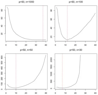
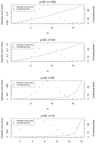
2.2 Operator norm errors and computing times with different choices ofm under Model (A) in Section2.10.1. . . 46

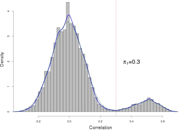
2.3 Determination ofπ1 by distribution of all the diagonal elements of the sample correlation matrix upon knowing the true covariance matrix is diagonal block matrix. π1 is chosen as the lowest point between two peaks. True covariance structure: σi,j = 1 fori = j, σi,j = 0.5for i6=j and{i, j} ⊆Aw,w∈(1,2,· · ·, W), and0else. . . 47

(14)

LIST OF FIGURES

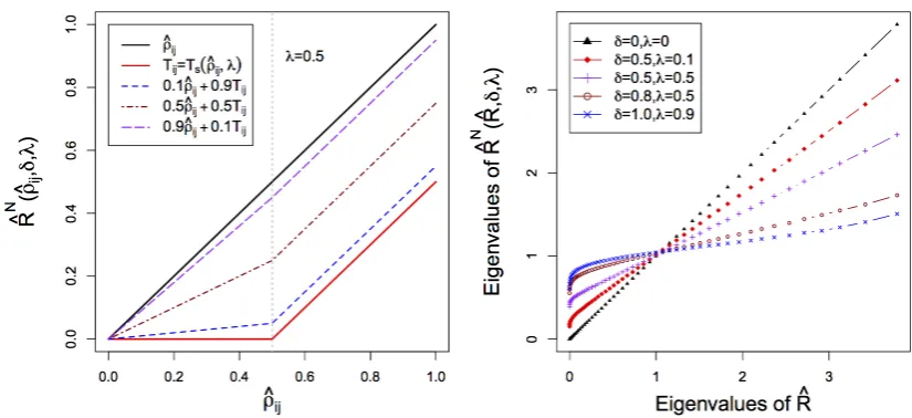
3.2 Left: Illustration of NOVELIST operators for any off-diagonal entry of the correlation matrixρˆijwith soft thresholding targetTs(λ = 0.5,δ=

0.1, 0.5 and 0.9). Right: ranked eigenvalues of NOVELIST plotted versus ranked eigenvalues of the sample correlation matrix. . . 77

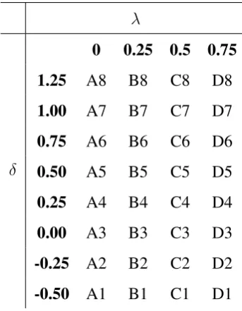
3.3 Robustness of(λ, δ)aspincreases for various choices of(λ, δ)(Table

3.1). Top left: NOVELIST (Model (E)); top right: NOVELIST (Model (F)); bottom left: PC-adjusted NOVELIST (Model (E)); bottom right: PC-adjusted NOVELIST (Model (F)),n= 100. . . 95

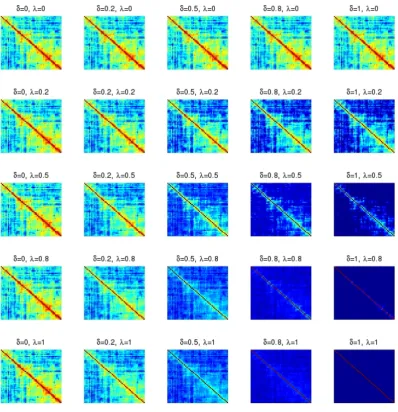
3.4 Image plots of operator norm errors of NOVELIST estimators of Σ

with different λ andδ under Models (A)-(C) and (G), n = 100, p = 10(Left),100(Middle),200(Right), simulation times=50. The darker the area, the smaller the error. . . 103

3.5 Image plots of operator norm errors of NOVELIST estimators of Σ

with differentλandδunder Models (D)-(F),n = 100,p= 10(Left),100

(Middle),200 (Right), simulation times=50. The darker the area, the smaller the error. . . 104

3.6 50 replicated cross validation choices of(δ0, λ0)(green circles) against the background of contour lines of operator norm distances toΣunder model (A), (C), (D) and (F) [equivalent to Figures 3.4 and3.5], n = 100,p= 10(Left),100 (Middle),200(Right). The area inside the first contour line contains all combinations of(λ, δ)for which||ΣˆN₍_{λ, δ}₎₋

Σ||is in the 1st decile of[[min (λ,δ)||

ˆ

ΣN₍_{λ, δ}₎₋_Σ_||,_[_max (λ,δ)||

ˆ

(15)

LIST OF FIGURES

4.1 Contour plots of proportions of the times when NOVELIST outper-forms in terms of the choices of (λ, δ) under rebalancing regime 1 (left column) and 2 (right column). “1” indicates the area of choices of (λ, δ)which makes NOVELIST to outperform with the chance of

100%, in contrast, “0” indicates the area of choices of (λ, δ) where NOVELIST never outperform. The suggested fixed parameter(λ00, δ00) = (0.75,0.50) for factor model which is used in Automatic NOVELIST algorithm in Section3.7is marked as a plus. . . 129

4.2 Distribution of Annualised sample variances and covariances of intra-day returns of the FTSE 100 constitutes from March 2nd 2015 to September 4th 2015. Sampling frequency=5,10,30minutes. . . 133

4.3 Time series plots of six minimal variance portfolio returns and STDs based on intra-day data. . . 135

4.4 Competitions of call forecasting based on forecast 1 to 3. Left: plots of average absolute errors for the forecasts using different estimators. Right: percentage of days (29 of them) in the test dataset when the NOVELIST based forecast outperforms for each ten-minute interval at later times in the day. . . 142

(16)

LIST OF FIGURES

4.6 The estimated false discovery proportion as function of the threshold valuetand the estimated number of false discoveries as function of the number of total discoveries for p = 3226genes in total. The number of factorsk ∈(2,15). . . 150

(17)

List of Tables

2.1 Comparison of precision estimators in Case I . . . 37

2.2 Means and variances (in brackets) of the precision matrix estimators from Case I . . . 38

2.3 Comparison of precision estimators in Case II(|Aw|= 2) . . . 41 2.4 Means and variances (in brackets) of the precision matrix estimators

from Case II(|Aw|= 2) . . . 41

2.5 Comparison of precision estimators in Case III(|K|= 1) . . . 44

2.6 Means and variances (in brackets) of the precision matrix estimators from Case III(|K|= 1) . . . 44

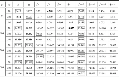
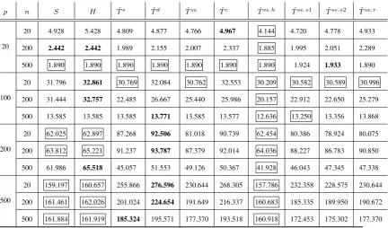
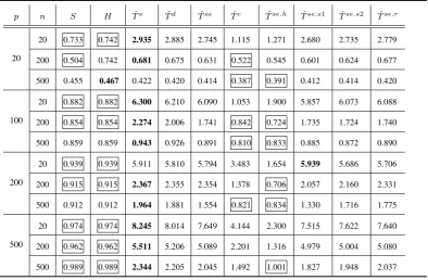
2.7 Average operator norm error for competing precision estimators with optimal parameters under model (A) (50 replications). The best results and those up to 5% worse than the best are boxed. The worst results are in bold. . . 55

(18)

LIST OF TABLES

2.9 Average operator norm error for competing precision estimators with optimal parameters under model (C) (50 replications). The best results and those up to 5% worse than the best are boxed. The worst results are in bold. . . 57

2.10 Average operator norm error for competing precision estimators with optimal parameters under model (D) (50 replications). The best results and those up to 5% worse than the best are boxed. The worst results are in bold. . . 58

3.1 Parameter choices for robustness tests . . . 94

3.2 Choices of(λ∗, δ∗)and(λ0, δ0)forΣˆN (50 replications). . . 101

3.3 Average operator norm error toΣfor competing estimators with opti-mal parameters (50 replications). The best results and those up to 5%

worse than the best are boxed. The worst results are in bold. . . 106

3.4 Average operator norm error toΣfor competing estimators with data-driven parameters (50 replications). The best results and those up to

5%worse than the best are boxed. The worst results are in bold. . . . 107

3.5 Average operator norm error toΣ−1for competing estimators with op-timal parameters (50 replications). The best results and those up to5%

worse than the best are boxed. The worst results are in bold. . . 108

3.6 Average operator norm error to Σ−1 _{for competing estimators with} data-driven parameters (50 replications). The best results and those up to5%worse than the best are boxed. The worst results are in bold. 109

(19)

LIST OF TABLES

4.1 Proportion of times (Nof them) when in-sample covariance matrix has prominent PCs or high-kurtosis off-diagonals and decisions of NOV-ELIST algorithm made according to Section3.7. . . 126

4.2 Annualised portfolio returns, standard deviations (STDs) and Sharpe ratios of minimum variance portfolios (based on daily data) as in for-mula (4.4). The best results are boxed. . . 128

4.3 Annualised portfolio returns, standard deviations (STDs) and Sharpe ratios of minimum variance portfolios (based on intra-day data) as in formula (4.6). The best results are boxed. . . 136

4.4 Allocation of training and test datasets for forecast 1 to 6. . . 139

4.5 Mean absolute forecast errors and standard deviations (in brackets) of forecast 1 to 6. The best results are boxed. . . 141

(20)

Chapter 1

Introduction

1.1

Literature review

Estimating the covariance matrix and its inverse, also known as the concentration or precision matrix, has always been an important part of multivariate analysis, and arises prominently. In particular, covariance matrix and its inverse play a central role in port-folio selection and financial risk management. The adequacy of diversification of a portfolio, which is highly related to “risk”, is quantified by the covariance matrix of the assets [Markowitz, 1952]. For example, the largest and smallest eigenvalues of the covariance matrix provide the boundary for the variance of return of each possible portfolio allocation [Fan et al.,2008;Markowitz,1952]. SeeLedoit and Wolf[2003],

Talih [2003], Goldfarb and Iyengar [2003] and Longerstaey et al. [1996] for appli-cations of covariance matrices to portfolio selection and financial risk management. Also, in principal component analysis, where eigenanalysis of covariance matrix is es-sential for computing principal components [Croux and Haesbroeck, 2000; Jackson,

(21)

where common or individual covariance matrix is inverted in discriminant function for classification or dimension reduction purposes [Bickel and Levina,2004;Fisher,1936;

Guo et al.,2007]. Moreover, graphical modeling [Meinshausen and B¨uhlmann,2008;

Ravikumar et al.,2011;Yuan,2010] with its applications in network science [Gardner et al., 2003; Jeong et al., 2001] require a good covariance matrix estimator inverting which does not excessively amplify the estimation error. Naturally, this is also true of the correlation matrix, and the following discussion applies to the correlation matrix, too. The sample covariance matrix is a straightforward and often used estimator of the covariance matrix [Anderson,1968]. However, estimating large covariance matrices is intrinsically challenging. When the dimensionpof the data grows with the sample size n, the sample covariance matrix is no longer a consistent estimate in the sense that its eigenvalues do not converge to those of the true covariance matrix, according to ran-dom matrix theory [Chen et al.,2013;Johnstone, 2001;Mar˘cenko and Pastur, 1967]. Moreover, sample precision matrix is not defined because sample covariance matrix is singular in the high-dimensional setting. Even if pis smaller than but of the same order of magnitude as n, the number of parameters to estimate isp(p+ 1)/2, which can significantly exceedn. In this case, the sample covariance matrix is not reliable, and alternative estimation methods are needed.

(22)

long as logp/n → 0under Gaussianity. Furrer and Bengtsson[2007] and Cai et al.

[2010] regularise estimated ordered covariance matrices by tapering.Cai et al.[2010] derive the optimal estimation rates for the covariance matrix under the operator and Frobenius norms, a result which implies sub-optimality of the convergence rate of the banding estimator of Bickel and Levina [2008a] in the operator norm. The banding technique is also applied to the estimated Cholesky factorisation of the inverse of the covariance matrices [Bickel and Levina, 2008a;Wu and Pourahmadi,2003]. Another important example of a structural assumption on the true covariance or precision ma-trices is sparsity; it is often made e.g. in the statistical analysis of genetic regulatory networks [Gardner et al.,2003;Jeong et al., 2001]. El Karoui[2008] andBickel and Levina [2008b] simultaneously and independently regularise the estimated sparse co-variance matrix by universal thresholding, which is a simple and permutation-invariant method of covariance regularization. El Karoui [2008] develops thresholding under a special notion of sparsity called β-sparsity, and Bickel and Levina [2008b] study thresholding under another class of sparse matrices, which is stronger and parallels to the class of the approximately “bandable” matrices in [Bickel and Levina, 2008a].

(23)

covari-ance and precision matrices [d’Aspremont et al.,2008;Friedman et al.,2008;Rothman et al.,2008;Yuan and Lin,2007;Zou, 2006]. Also,Fan and Li[2007];Lam and Fan

[2009];Zhao and Yu[2001] addresses explicitly the issues of sparsistency and the bias problem due toL1 penalization. Upon sparsity assumption, a closely related problem is the estimation of the support of the precision matrix which corresponds to the se-lection of graphical models for Gaussian distributions [Lauritzen,1996]. Focusing on model selection rather than parameter estimation,Meinshausen and B¨uhlmann[2008] propose the neighbourhood selection method with the Lasso technique for estimating the pattern of zero entries in the precision matrix of a multivariate normal distribution, based on which Peng et al. [2009] develop a faster algorithm to select the non-zero partial correlations by using a joint sparse regression model. One other commonly oc-curring structural assumption in covariance estimation is the factor model, often used e.g. in financial applications. Motivated by the Arbitrage Pricing Theory in finance,

Fan, Fan, and Lv[2008] impose a multi-factor model on data to reduce dimensionality and to estimate the covariance matrix, where the factors are observable and the number of factors can grow with dimensionp. Fan et al.[2013] propose the POET estimator, which assumes that the covariance matrix is the sum of a part derived from a factor model, and a sparse part.

(24)

leave the sample eigenvectors unchanged. However, Ledoit and P´ech´e [2011] argue that the differences between the eigenvalues of the sample covariance matrix and those of the population covariance matrix are highly nonlinear and derive the asymptoti-cally optimal bias correction for sample eigenvalues. Based on it, Ledoit and Wolf

[2012] extend linear shrinkage to nonlinear shrinkage of the eigenvalues of the sam-ple covariance matrix. Ledoit and Wolf [2013] also derive a consistent estimator of the oracle nonlinear shrinkage based on the consistent estimation of the population eigenvalues (also known as the spectrum). Lam [2016] introduces a Nonparametric Eigenvalue-Regularized Covariance Matrix Estimator (NERCOME) through subsam-pling of the data, which is asymptotically equivalent to the nonlinear shrinkage method of Ledoit and Wolf[2012]. Shrinkage can also be applied on the sample covariance matrix directly. Ledoit and Wolf[2003] propose a weighted average estimator of the covariance matrix with a single-index factor target to account for common market co-variance and provide analytic calculation of the optimal shrinkage intensity. Schäfer and Strimmer [2005] review six different shrinkage targets and derive improved co-variance estimator based on the optimal shrinkage intensity inLedoit and Wolf[2003]. Besides, shrinkage techniques are also used for spectral analysis of multivariate time series of high dimensionality. Böhm and von Sachs[2008] shrink the empirical eigen-values in the frequency domain towards one another to improve upon the smoothed periodogram as an estimator for the multivariate spectrum. Also,Böhm and von Sachs

[2009] propose a nonparametric shrinkage estimator of the spectral matrix which has asymptotically minimal risk among all linear combinations of the identity and the av-eraged periodogram matrix. Naturally related to the shrinkage approach is Bayesian estimation of the covariance and precision matrices. Evans[1965], Chen[1979], and

(25)

matrix of a multivariate normal distribution, the inverted Wishart distribution. More-over, Leonard and John [2012] propose a flexible class of covariance matrix prior, which yields more general hierarchical and empirical Bayes smoothing and inference.

Alvarez [2014] proposes some alternative distributions, including the scaled inverse Wishart distribution, which gives more flexibility on the variance priors, and separate priors for variances and correlations, which eliminates any prior relationship among covariance matrix elements.

1.2

Organization and Outline of the thesis

The thesis is structured as follows. In Chapter2we propose tilting-based precision ma-trix estimators of ap-dimensional random variable,X, whenpis possibly much larger than the sample sizen. Four types of tilting-based methods are introduced and the rate of convergence are addressed under certain assumptions. Asymptotic properties of the estimators are studied whenpis fixed andpgrows withn. For finitepandn, extensive comparisons of thresholding estimators and the proposed methods are demonstrated. Several improvement approaches are made. The simulation results are presented under different models.

(26)

algorithm) is presented. Further empirical improvements of NOVELIST are proposed. Comprehensive simulation study is based on a wide range of models and results of comparisons with several popular estimators are presented. Finally, an automatic al-gorithm is constructed to provide an adaptive choice between the use of LW-CV algo-rithm and fixed parameters.

Chapter4is devoted to explore the applications of NOVELIST estimators and to exhibit the results of applying the estimators on real data, including portfolio opti-mization using low-frequency and high-frequency FTSE 100 constituents log returns, forecasting the number of calls for a call center and estimating false discovery propor-tion through a well-known breast cancer study. Chapter5concludes the thesis.

1.3

Conclusion

(27)

Chapter 2

Precision Matrix Estimation via tilting

2.1

Introduction

For multivariate normal distributions, the support of the estimate of the precision ma-trix is closely related to graphical models. For graphical models, each node corre-sponds to a random variable, and each non-zero edge between two nodes represents conditional dependence between the corresponding random variables after removing the effects of all the other variables. In this chapter, we consider ap-dimensional mul-tivariate normal distributed random variable X = (X1, X2,· · ·, Xp)withn i.i.d. ob-servations,P={1,2,· · ·, p},EX = 0, covariance matrix isΣ ={σi,j}=E(XTX), and precision matrix isΣ−1 ₌_P ₌_{p

(28)

par-tial correlations between corresponding variable pairs conditional on the rest of the variables, as partial correlation betweenXiandXj is defined asρ˘i,j =

−pi,j

√

pi,i√pj,j [Peng et al.,2009], which is very useful in estimation in Gaussian graphical models.

There exists a well-known link between partial correlations and regression models under Gaussianity, based on which a partial correlation estimation method is intro-duced by Peng et al.[2009]. Although it is not directly linked to this work, it gives us inspiration for exploring the relationship between precision matrix and regression models, based on which our work is carried on. For given i, by regressionXi on all the other variables inP, we have

Xi =

X

j∈P\{i}

βi,jXj +ζi, (2.1)

where ζi are uncorrelated with each Xj, j ∈ P \ {i}. From Lemma 1 in Peng

et al. [2009], we have βi,j = ˘ρi,j

q_p j,j

pi,i. Analogously, by regression Xj on all the

other variables, we also have βj,i = ˘ρj,i

q_p i,i

pj,j. Since ρ˘i,j = ˘ρj,i, we obtain ρ˘i,j =

sign(βi,j)

p

βi,jβj,i. Therefore, the search for non-zero partial correlations, i.e. deter-mining the non-zero edges in graphical models, can be viewed as a model selection problem under the Gaussian regression settings.

However, we aim to estimate the precision matrix, which is closely related to the partial correlations but cannot be explicitly expressed by them. Instead, we find another way to link ap×pprecision matrixΣ−1_{to regression models block by block as follows.} For simplicity, we choosep= 3for illustration.

(29)

matrix, and denoted byΣ◦_i,j−1, where

Σ−1 =

      • • · • • · · · ·      

←i= 1

←j = 2, (2.2)

Σ◦_1,2−1 =.

   • • • •   =cov

−1₍_X

1,X2|X−(1,2)). (2.3) Here, cov(X1,X2|X−(1,2))is a partial covariance matrix, i.e. the covariance matrix ofX1 andX2 given all the other variables. Formula (2.3) indicates that the pairwise precision matrix Σ◦_1,2−1 _{equals the inverse of the pairwise partial covariance matrix.} Since partial covariance matrix can be estimated by using regression models, precision matrix estimation is linked to regression problems. More detailed explanation about this comes later.

Step two: fori = 1andj = 3, we obtain another four elements ofΣ−1 _(indicated as green dots).

Σ−1 =

      • • • • • · • · •      

←i= 1

←j = 3,

(2.4)

Σ◦_1,3−1 =.

   • • • •   =cov

−1₍_X

1,X3|X−(1,3)), (2.5) where, cov(X1,X3|X−(1,3)) is the partial covariance matrix ofX1 andX3 given all the other variables.

(30)

all the entries of Σ−1. We note that each diagonal involves (p−1)different 2 by 2 blocks asiandj move around across all indices, we use their average values finally.

Now, we focus on formula (2.3) and explain how the last equality is obtained. Actually it comes from the block-wise inversion of matrix [Bernstein,2009, p.147] as follows,



 

A B

BT C

   −1 =   

(A−BC−1BT)−1 −(A−BC−1BT)−1BC−1

−C−1_BT₍_A₋_BC−1_BT₎−1 _C−1₊_C−1_BT₍_A₋_BC−1_BT₎−1_BC−1



 ,

(2.6)

whereA,BandCare matrix sub-blocks of arbitrary size,AandC must be square,C andA−BC−1_BT _{must be nonsingular. The proof of formula (}_2.6_{) is given in Section}

2.12.1. We note that,A−BC−1BT is actually in a form closely related to conditional covariance. For illustration, we give a simple example of a 3 by 3 sample precision matrixΣˆ−1 of a multivariate normal random variableX = (X1, X2, X3)withni.i.d. observations,Σˆ−1 ₌_XT_X_{. We partition}_Σ_ˆ−1_{and apply the top-left part (indicated in} red) of the right-hand side of formula (2.6) on it, which leads to

ˆ Σ−1 =

      ˆ

σ1,1 σˆ1,2

ˆ

σ2,1 σˆ2,2

ˆ

σ1,3

ˆ

σ2,3

ˆ

σ3,1 σˆ3,2 σˆ3,3

      −1 =           ˆ

σ1,1−σˆ1,3σˆ3−,13σˆ3,1 σˆ1,2−σˆ1,3σˆ3−,31σˆ3,2 ˆ

σ2,1−σˆ2,3σˆ3−,13σˆ1,3 σˆ2,2−σˆ2,3σˆ3−,31σˆ3,2    −1 · · · · ·        , (2.7)

(31)

that this part corresponds to the inverse of the pairwise sample conditional covariance matrix of(X1, X2)givenX3. For example, we note that

ˆ

σ1,2−σˆ1,3σˆ3,3−1σˆ3,2

=X₁TX2−X₁TX3(X₃TX3)−1X₃TX2

=X₁T(In−H3)X2

=cov_c((In−H3)X1,(In−H3)X2)

=cov_c(X1|X3, X2|X3), (2.8)

where In is a n by n diagonal matrix, H3 is the projection matrix onto the space spanned byX3,H3

.

=X3(X3TX3)−1X3T andcovc(X1|X3, X2|X3)is the sample

condi-tional covariance betweenX1 andX2 givenX3, which can be obtained by computing the sample covariance between the residuals of regressing X1 and X2 on X3. When

ˆ

Σ−1is partitioned in different combinations of the indices, the results of the remaining part of formula (2.7) (indicated as dots) will be obtained. Actually, this relationship is also true at the population level, which means that any 2 by 2 block indexed by

(i, j)of any precision matrix is equivalent to the inversion of the pairwise conditional covariance matrix of (Xi, Xj) given all the other variables, see Lemma1 in Section

(32)

to the large dimensionality and possibly strong collinearity among the remaining vari-ables. Also, in high dimensional geometry, even when variables follow independent Gaussian distributions, spurious sample marginal correlations among variables would be observed [Fan and Lv,2008], leading to wrong regression models. Over the last two decades, substantial efforts have been made in tackling this high-dimensional variable selection problem. An exhaustive review can be found inFan and Lv[2010] under the assumption that regression coefficients are assumed to be sparse with many being zero. Among them, one of the intensively studied area is the penalised least squares estima-tion, such as the Lasso [Tibshirani, 1996], the ridge regression, the SCAD [Fan and Li, 2007] and their extensions [Meinshausen, 2007; Zou, 2006]. Fan and Lv [2008] introduce the Sure Independence Screening (SIS), which ranks the importance of each variable according to the magnitude of the corresponding marginal correlation between the variable and the response, and selects the firstdnvariables which have the largest magnitude of correlations. SIS reduces the dimensionality from high or ultra high (for example,logp= O(na₎_{for some}_{a >} ₀_{) to the scale}_d

n, which can be less thann, in a computationally efficient way.

(33)

algo-rithm, where partial correlation instead of marginal correlation is applied in order to iteratively remove irrelevant variables from the model. Cho and Fryzlewicz [2012] introduced tilted correlation to measure the strength association between the variables and the response which takes into account collinearity. The tilted correlation is closely related to partial correlation, but it focuses on regressing the responseY on the vari-ablesXk, and thusY andXkare not treated on an equal footing. For any given variable Xk,k ∈P, the tilted correlation is designed to capture the linear relationship between Xk and the responseY, after removing the effects of all the highly related remaining variables (not all the other variables), onXkonly instead of on bothXkandY. A more detailed explanation of the tilted correlation can be found in Section2.2.

Motivated by the link between precision matrix and regression models, this chapter proposes tilting techniques which are applied to simultaneously select the (hopefully) highly relevant remaining variables for each pair Xi and Xj when p grows with n, which leads to block by block large precision matrix estimation . To tackle the si-multaneous variable selection problems for high-dimensional regression models, we introduce four types of tilting methods. The first three methods rely on ranking of the marginal correlations, while the last one apply tilted correlations in order to remove or reduce the effects of collinearity. We investigate the asymptotic properties of the tilting estimators under suitable assumptions as well as small sample inference. Furthermore, empirical choices of parameters and improvements are discussed and algorithms are listed for the estimators. Also, simulation studies are presented afterwards.

(34)

matrix, and illustrate the motivation by a simulation example. In Section 2.4, tilt-ing methodology is formally defined and four types of tilttilt-ing methods are introduced. Section 2.5 lists the algorithms for the tilting estimators. Section 2.6 establishes the consistency of the tilting estimators under assumptions for fixedpand whenpgrows with n. Section2.7 analytically investigates the finite sample performance of tilting estimators and the differences and links between the tilting estimators and soft and hard thresholding estimators. Section2.8gives suggestions on choices of parameters. Section 2.9 exploits optional empirical improvements of the tilting estimators. Sec-tion2.10exhibits practical performances of the tilting estimators in comparison to the thresholding estimators. Section2.11concludes the chapter. Section2.12is additional lemmas and proofs.

2.2

Preliminary:

tiltied correlation

Before introducing the proposed methods for precision matrix estimation, we need to briefly describe what is the so called “tilted” correlation introduced by Cho and Fryzlewicz[2012] and how it works. It considers the following linear model:

Y =Xβ+, (2.9)

(35)

The marginal correlation between each variableXk and Y can be written as the following decomposition,

X_kTY =X_kT(

p

X

s=1

βsXs+) = βk+

X

s∈S\{k}

βsXkTXs+XkT, (2.10)

which shows that marginal correlation screening is not reliable on selecting S if the underlined summand in formula (2.10) is non-negligible. For example, irrelevant vari-ables that are highly related with the relevant ones can be selected by using marginal correlation screening. Also, if high collinearity exists among the variables, the results coming from marginal correlation screening could be far away from the true setS. It can even be the case that the relevant variables are ruled out when marginal correlation screening is applied. Consider the following example,

Y =βX1+βX2−2β √

ϕX3+, (2.11)

where ∼ N(0,In)and(X1, X2, X3)T are generated from a multivariate normal dis-tribution N(0,Σ) independently for i = 1,2,3. The population covariance matrix

Σ = {σi,j} satisfies σi,i = 1 and σi,j = ϕ, i 6= j, except σi,3 = √

ϕ. It is clear that corr(X3, Y) = 0, which indicates that X3 is marginally uncorrelated with Y at the population level, and is likely to be ruled out if marginal correlation screening is applied, butX3is actually a relevant variable with Y.

(36)

the tilted variableX_k∗for eachXk, which is defined as

X_k∗ = (. In−Hk)Xk, (2.12) whereHk is the projection matrix onto the space spanned byXek, i.e. Hk

.

=X_e_k(XT ek

X_e_k)−1XT

e

k, and Xek is a submatrix of XP\{k}, which contains all the remaining vari-ables that are highly correlated withXk. It is clear that the tilted variable is a projected version of the original one, which removes the effects of all the highly correlated vari-ables.

Then the tilted correlation is introduced based on the tilted variable. We can de-compose(X_k∗)T_Y _as

(X_k∗)TY =X_kT(In−Hk)Y =XkT{ p

X

s=1

βs(In−Hk)Xs+ (In−Hk)}

=βkXkT(In−Hk)Xk+

X

s∈_S\{ek},s6=k

βsXkT(In−Hk)Xs+XkT(In−Hk) (2.13)

If we rescale(X_k∗)T_Y _{by dividing}_XT

k(In−Hk)Xk (rescaling 1 inCho and

Fry-zlewicz [2012]), and as long as the second and the third summands in formula (2.13) are negligible in comparison with the first, the rescaled tilted correlation can be rep-resented as βk plus a small term. We denote ak

.

= kHkXkk 2

2/kXkk 2

2, then we have

1−ak = XkT(In −Hk)Xk as the rescaling factor of making the norm of the tilted correlation to be 1. From now on, we refer to “tilted correlation” as the rescaled tilted correlation, and denote it bycorr_d∗.

(37)

the underlined term in formula (2.13) is negligible. For example, condition 1 inCho and Fryzlewicz[2012] means that ifXsis not highly relevant toXkitself, it remains not highly relevant to the projectedXk onto the space spanned byX_e_k, i.e. HkXk, which can be shown to hold asymptotically when each columnXkis generated independently as a random vector on a sphere of radius 1, which is the surface of the Euclidean ball Bn

2 ={x∈Rn :

Pn i=1x

2

i 61}by using Lemma4in Section2.12.2.

To sum up, the tilted correlation measures the rescaled correlation between the responseY and the tilted version of the variableXi that removes the effects of all the highly relevant remaining variables onXi. More explanations regarding how it can be applied to precision matrix estimation come later in Section2.4.2.4and the algorithm can be found in Section2.5.2.

2.3

Notations, building block and motivations

2.3.1

Notations and building block

Σ

ˆ

◦₂_×₂−1

For a given pair ofiandj,i, j ∈ P, we denoteK = P\ {i, j}. If we partitionX as

(Xij,X−(ij)), whereXij = (Xi, Xj), X−(ij) = (Xk : k ∈ K), the covariance matrix

Σis decomposed as follows,

Σ =



 

Σ2×2 Σ2×(p−2)

Σ(p−2)×2 Σ(p−2)×(p−2)



 

p×p

, (2.14)

where Σ2×2 = E(XijTXij), Σ2×(p−2) = E(XijTX−(ij)), Σ(p−2)×2 = E(X−T(ij)Xij),

(38)

parti-tioned as

P =



 

Σ2×2 Σ2×(p−2)

Σ(p−2)×2 Σ(p−2)×(p−2)



 

−1

p×p

=



 

P2×2 P2×(p−2) P(p−2)×2 P(p−2)×(p−2)



 

p×p

. (2.15)

Lemma 1 IfX ∼ N(0,Σ),ΣandP are partitioned as in formula (2.14) and (2.15), andΣ(p−2)×(p−2) andΣ2×2−Σ2×(p−2)Σ−_(p1−2)×(p−2)Σ(p−2)×2 are nonsingular, then

P2×2 = (Σ2×2−Σ2×(p−2)Σ−(p1−2)×(p−2)Σ(p−2)×2)−1 =cov−1(Xij|X−(ij)), (2.16)

whereXij = (Xi, Xj).

The first equality follows because of the block-wise inversion of matrix (formula (2.6) in Section2.1). The second equality follows due to properties of marginal and condi-tional normal distribution [Tong,2012, p.35].

Lemma1shows thatP2×2 is not the inversion ofΣ2×2, instead, it is the inversion

of the 2 by 2 pairwise conditional covariance matrix which we define as

Σ◦₂_×₂ =. cov(Xij|X−(ij)), (2.17) where Xij = (Xi, Xj). i.e. Σ◦2×2 is the covariance matrix of Xi andXj controlling all the other variables, X−(ij), for estimating which, the natural way in practice is to regressXiandXj on all the other variables.

By regressingXiandXj on all the other variables,X−(ij), respectively, we obtain 2 simultaneous regression models

Xi =

X

k∈_K

(39)

Xj =

X

k∈_K

βj,kXk+j, (2.19)

wherei andjare specific terms ofXiandXjrespectively,E(i) =E(j) = 0,Xkis uncorrelated withiandj. We denoteij = (i, j), hence we have cov(ij) = Σ◦2×2. In order to estimateP2×2, we need to replaceij byˆij. Typically,ˆij can be obtained by Least Squares Estimation,

ˆ

i = (In−H−(ij))Xi, (2.20)

ˆ

j = (In−H−(ij))Xj, (2.21) i.e. ˆij = (In−H−(ij))Xij. Then we obtainΣˆ2◦×2 = covc(ˆij), andPˆ2×2 = ˆΣ

◦

2×2

−1_. Furthermore, asiandj move around across all indices inP, each pair ofiandjyields itsΣˆ◦₂_×₂−1_{, which fills in the corresponding elements of the precision matrix estimator,} and eventually the estimation of the entire precision matrix P is obtained. It is clear thatΣˆ◦₂_×₂−1is the building block of the precision matrix estimator.

However, we note that the building block does not have to be a 2 by 2 matrix. If we denote S as a subset of P, K = P\S, |S| = m and|K| = p−m. In general, for any m satisfying 2 ₆ m < min(p, n), the link between precision matrix and regression models still exist. Now, we describe the links between precision matrix and regression models in the general notations. We partition X as(X_S,X−_S), where

X_S = (Xs : s∈ S),X−_S =X_K = (Xk :k ∈K). The partitioned covariance matrix is

Σ =



 

Σm×m Σm×(p−m)

Σ(p−m)×m Σ(p−m)×(p−m)



 

p×p

(40)

and the partitioned precision matrix is

P =



 

Pm×m Pm×(p−m) P(p−m)×m P(p−m)×(p−m)



 

p×p

, (2.23)

By respectively regressingX_S on all the other variablesX−_S, we obtainm

simultane-ous regression models. We denote the specific terms _S as_S = (s : s ∈ S). Since m < n, the projection matrixH−S =X−S(X−TSX−S)−1X−TS is well defined. Hence,

we obtainˆ_S = (In−H−S)XS and

ˆ

Σ◦_m_×_m =cov_c(ˆ_S), (2.24)

ˆ

Pm×m = ˆΣ◦m×m

−1_.

(2.25)

(41)

2.3.2

Motivation and example illustrations

Choosing|S|= 2means that|K|=p−2. Whenpn,Kinvolves too many variables such that the projection matrix H−S is not well-defined and regression coefficients

[image:41.595.145.466.352.661.2]

cannot be solved. Even if n > p but n is close to p, putting all the other variables in the regression models will also distort the estimators. To tackle this problem, it appears natural to replaceX_K by a controlling subsetX_C, where|C|is not bigger, in most cases much smaller than|K|, andX_C hopefully only contains the highly relevant controlling variables. Figure2.1 shows that the optimal size of the controlling subset

Figure 2.1: Frobenius norm errors ofΣˆ◦₂_×₂−1toP2×2with different size of the control-ling subsets under model D in Section2.10.1, X-axis is the size of controlling subsets |C|, Y-axis is the average Frobenius norm error of Σˆ◦₂_×₂−1 _to _P

(42)

is much smaller than|K|in most of the cases unlessn p.

Since, there are 2 regression models to be solved at the same time, the determina-tions of 2 controlling subsets forXiandXj are made simultaneously, which makes the problem more difficult. In the following section, we will introduce the tilting meth-ods of regularizing the controlling subsets forXi andXj which take into account the effects of the relationship betweenXiandXj on them.

2.4

Definitions and methods

2.4.1

Definitions

In this section, we formally introduce and define the precision matrix estimation via tilting. It is defined as

ˆ

T ={_tˆ_i,j_}, _{i, j} _∈_P_, _(2.26)

where

ˆ

ti,j =



 

 

[ ˆΣ◦_ij−1_]

1,2 ifi6=j 1

p−1

P

l∈P\{i}[ ˆΣ ◦

il

−1_]

1,1 ifi=j

, (2.27)

ˆ

Σ◦_ij is an alternative notation to Σˆ◦₂_×₂ with emphasis on the indices, Σˆ◦_ij = cov_c(X_ij∗), whereX_ij∗ = (Xi|X_Ci, Xj|XCj), XCi andXCj are the controlling subsets forXi and

(43)

(p−1)different 2 by 2 blocks asiandj move around across all indices inP, we use the average value as the final estimate of each diagonal.

2.4.2

Four types of tilting methods

One key ingredient of this methodology is simultaneous choice of the sets Ci andCj forXiandXj, which is the essential for the building blockΣˆ◦2×2, especially in

high-dimensional cases. Now, four types of tilting methods are introduced for determining the setsCiandCj, which can be identical to each other.

For each pair of specified indicesiand j, we can decompose formula (2.18) and (2.19) as follows,

Xi =

X

b∈_B

βi,bXb+

X

ei∈Ei

βi,eiXei+ X

ej∈Ej

βi,ejXej + X

u∈_U

βi,uXu+i, (2.28)

Xj =

X

b∈_B

βj,bXb +

X

ei∈Ei

βj,eiXei+ X

ej∈Ej

βj,ejXej+ X

u∈_U

βj,uXu+j, (2.29)

where

B={b:βi,b 6= 0,andβj,b 6= 0}, i.e. eachXb is a predictor for bothXi andXj; Ei ={ei :βi,ei 6= 0,andβj,ei = 0}, i.e. eachXei is a predictor forXi, but notXj;

Ej ={ej :βi,ej = 0,andβj,ej 6= 0}, i.e. eachXej is a predictor forXj, but notXi;

U = {u : βi,u = 0,andβj,u = 0}, i.e. none of Xu is a predictor for eitherXi or Xj;

i, andj are uncorrelated with eachXb,Xei,Xej andXu.

(44)

computationally fast. We note that the marginal correlation between variableXk and Xi, for example ifk∈B, has following decomposition,

X_kTXi =XkT(

X

b∈_B

βi,bXb+

X

ei∈Ei

βi,eiXei + X

ej∈Ej

βi,ejXej + X

u∈_U

βi,uXu+i)

=βk,i+ (

X

b∈B\{k}

βi,bXkTXb+

X

ei∈Ei

βi,eiX

T

kXei) +X

T

ki, (2.30)

which shows that marginal correlation between two variables is the corresponding re-gression coefficient plus bias terms (in bracket). But we will show in Section 2.6.2

that under certain assumptions, the bias terms would not contaminate consistency of the tilting estimators at element-wise level. The last tilting method applies tilted corre-lations [Cho and Fryzlewicz, 2012] instead of marginal correlations in order to make such bias terms zero or negligible.

2.4.2.1 Simple tilting

Simple tilting puts the variables which are highly correlated with eitherXi orXj into the controlling subsetX_Cs

i andXCsj, whereC

s

i andCsj are defined as

Cs i =C

s j =C

s

ij ={c:|corrd(Xc, Xi)|> π1 or |corrd(Xc, Xj)|> π1, c∈K}, (2.31)

where π1 is a threshold, π1 ∈ (0,1). Actually, Cs_ij intends to capture B∪Ei ∪Ej. Subject to |B|+|Ei|+|Ej| < n, after controllingXB∪Ei∪Ej for both Xi andXj, the

remaining parts are

Ri =

X

u∈_U

(45)

Rj =

X

u∈_U

βj,uXu+j. (2.33)

And their covariance can be written as

cov(Ri, Rj) = cov(

X

u∈U

βi,nXn,

X

u∈U

βj,uXu) +cov(i, j). (2.34)

2.4.2.2 Double tilting

Double tilting only controls the variables which are highly correlated with bothXiand Xj. Cd_i andCd_j are defined as

Cd

i =Cdj =Cdij ={c:|corrd(Xc, Xi)|> π1 and |corrd(Xc, Xj)|> π1, c ∈K}. (2.35)

It is clear that double tilting intends to control the variables inX_B. Subject to|B|< n, only controllingX_Bfor bothXiandXj, the remaining terms are

Ri =

X

ei∈Ei

βi,eiXei + X

ej∈Ej

βi,ejXej + X

u∈U

βi,uXu+i, (2.36)

Rj =

X

ei∈Ei

βj,eiXei+ X

ej∈Ej

βj,ejXej+ X

u∈U

βj,uXu+j. (2.37)

Then the corresponding covariance is

cov(Ri, Rj) =cov(

X

ei∈Ei

βi,eiXei+ X

ej∈Ej

βi,ejXej + X

u∈U

βi,uXu,

X

ei∈Ei

βj,eiXei

+ X

ej∈Ej

βj,ejXej + X

u∈_U

(46)

2.4.2.3 Separate tilting

Separate tilting applies different controlling subsets onXi andXj, i.e. Csei 6=Csej . We defineCse_i andCse_j as follows,

Cse

i ={ci :|corrd(Xci, Xi)|> π1, ci ∈K}, (2.39)

Cse

j ={cj :|corrd(Xcj, Xj)|> π1, cj ∈K}. (2.40)

We viewB∪EiandB∪Ej as the population-level counterparts ofCsei andCsej respec-tively. If we assume that|B|+|Ei|< nand|B|+|Ej|< n, the remaining summands after controllingX_B∪Ei forXiandXB∪Ej forXj respectively can be written as

Ri =

X

ej∈Ej

βi,ejXej + X

u∈U

βi,uXu+i, (2.41)

Rj =

X

ei∈Ei

βj,eiXei+ X

u∈U

βj,uXu+j, (2.42)

followed by expressing the covariance as

cov(Ri, Rj) =cov(

X

ej∈Ej

βi,ejXej+ X

u∈_U

βi,uXu,

X

ei∈Ei

βj,eiXei+ X

u∈_U

βj,uXu

+cov(i, j) (2.43)

2.4.2.4 Competing tilting

(47)

regulariza-tion ofCc_i andCc_j. We name it as “competing tilting” because at each iteration step, it determines a subset which includes correlated variables and lets them compete to each other according to the conditional correlations between each variable and the response given all the other variables within the subset. We recall the tilted correlationcorr_d∗ in Section2.2, and define the controlling subsets for competing tilting as follows,

Cc

i ={ci :|corrd

∗

(Xci, Xi)|> π1, ci ∈P}, (2.44)

Cc

j ={cj :|corrd

∗

(Xcj, Xj)|> π1, cj ∈P}. (2.45)

Competing tilting is highly related to separate tilting, as both aim to capture the sets B∪EiandB∪Ej.

For any remaining variableXk,k ∈ K, we denotesXek as a submatrix ofXK\{k}, which containsX_e_k,ek ∈ C_kas its columns, and each of them is highly correlated with

Xk, i.e. Ck = {ek : corr_d(X

e

k, Xk) > πn}. For considering the linear relationship betweenXiandXkafter removing the effects ofX_e_k, the tilted correlation betweenXi andXkafter appropriate rescaling method (rescaling 1 inCho and Fryzlewicz[2012]) is defined as

d

corr∗(Xk, Xi) = (1−ak)−1XkT(In−Hk)Xi, (2.46) where1−akis the rescaling factor of making the norm of the tilted correlation to be 1, ak

.

= kHkXkk2₂/kXkk2₂, Hk is the projection matrix onto the space spanned byXek,

Hk .

= X

e k(X

T e kXek)

−1_XT e

(48)

2.5

Algorithm of the tilting estimators for precision

ma-trix

2.5.1

Separate tilting

Here we list the algorithm of the separate tilting estimator. The simple and double tilting estimators can be achieved in the similar manner.

Step 1: Estimate the pairwise precision matrices by applying the separate tilting.

Step 1.1: For a given pair of (i, j), and a chosen threshold π1, determine the controlling subsets Cse_i = {ci : |corrd(Xci, Xi)| > π1, ci ∈ K} and C

se

j = {cj : |corr_d(Xcj, Xj)|> π1, cj ∈K}.

Step 1.2: Compute the pairwise precision matrix ( ˆΣ◦_ij)−1 ₌ 1 nXi

T₍_I n −

Xci(X

T ciXci)

−1_XT

ci)(In−Xcj(X

T cjXcj)

−1_XT cj)Xj.

Step 1.3: Repeat 2.1-2.2 for all the combination ofiandj.

Step 2: Construct the precision matrix estimation.

Step 2.1: For off-diagonal entries,tˆse

i,j = [( ˆΣ◦ij)−1]1,2

Step 2.2: For diagonal entries,ˆtse_i,j = _p₋1₁ P

j6=i[( ˆΣ

◦

ij)−1]1,1

2.5.2

Competing tilting and the TCS algorithm

The only difference between separate tilting and competing tilting is in Step 1.1, where the marginal correlation corr is replaced by the tilted correlation_d corr_d∗ for competing tilting. The tilted correlation screening algorithm (TCS algorithm) is described in Sec-tion 3.1 of Cho and Fryzlewicz [2012]. Below, we list the algorithm which is taken from the paper to make the contents of the thesis coherent and easy to follow.

(49)

Rn _{is an} _{n-vector of the response,} _β ₌ _{β

1, β2,· · ·, βp} is the coefficient vector,

X = (X1, X2 · ··, Xp) is an n × p design matrix and % = (%1,· · ·, %n)T ∈ Rn is an n-vector of i.i.d. random errors, the aim of the TSC algorithm is to determine an active set denoted asA, that contains the real relevantXvariables toyafter effectively removing the non-negligible effects of all the otherX variables, i.e. according to the tilted correlationcorr_d∗betweenXvariables andy.

Step 0: Start with an empty active setA =∅, current residualz = y, and current design matrixZ =X.

Step 1: Find the variable which achieves the maximum marginal correlation with z and letk = arg max_{j /}_∈_A|ZT

j z|. IdentifyCk = {j /∈ A, j 6= k : |ZjTz| > πn}and if Ck =∅, letk∗ =kand go to Step 3.

Step 2: IfCk 6=∅, screen the tilted correlations betweenZj andz, corrd

∗

(Zj, z)in formula (2.46), forj ∈Ck∪ {k}and findk∗ =arg maxj∈_Ck∪{k}|corrd

∗

(Zj, z)|.

Step 3: Addk∗ toAand update the current residual and the current design matrix

z ← (In −HA)y and Z ← (In −HA)X, respectively, whereHA the projection matrix of Xk, k ∈ A, i.e., HA

.

= X_A(X_ATX_A)−1X_AT. Further, rescale each column j /∈AofZ to have norm one.

(50)

2.6

Asymptotic properties of tilting methods

2.6.1

Fixed

p

: asymptotic properties of

Σ

ˆ

◦_m_×_m−1

In this section, we briefly show the consistency of the building block of the estimators in the generalized form, i.e. Σˆ◦_m_×_m−1defined in formula (2.24)-(2.25), whenpis fixed. Here, the controlling subsets contain all the other variables, that is to say, for fixed p, it is safe to include all the remaining variables in the controlling subsets as long asnis large enough.

Lemma 2 Consistency: Ifp <∞and2₆m < p, thenΣˆ◦_m_×_m−1 →p Pm×m.

Proof of Lemma 2: Since each Xi, i ∈ P, follows i.i.d. Gaussian distribution with mean zero and finite variance, by the weak law of large numbers [Davidson, 1994, p.289], we note thatX_STX_S →p Σm×m,X−TSXS

p

→Σ(p−m)×m,X_STX−S

p

→Σm×(p−m),

XT

−SX−S

p

→ Σ(p−m)×(p−m). By Slutsky’s Theorem [Serfling, 2009, p.19] and the

block-wise inversion of covariance matrix [Bernstein,2009, p.147], we obtain

ˆ

Σ◦_m_×_m−1 = (ˆT_Sˆ_S)−1

= (X_ST(I −H−_S)X_S)−1

= (X_STX_S−X_STX−S(X−T_SX−S)−1X−T_SXS)−1

p

→(Σm×m−Σm×(p−m)Σ_(p−1−m)×(p−m)Σ(p−m)×m)

−1

=Pm×m (2.47)

(51)

2.6.2

p

→ ∞

: assumptions and consistency

2.6.2.1 Assumptions

In studying the theoretical properties of the four types of tilting methods for estimating precision matrices, we make the following assumptions and also give the reasons for and examples satisfying these assumption.

A. 1 For any i, j ∈ Pin formula (2.28) and (2.29), we assume Xb, Xei, Xej, Xu, i andj are mutually uncorrelated.

Assumption (A.1) is made in order to ensure element-wise consistency of the precision matrix via all the four types tilting methods. Although it seems a strong assumption, we can find examples which satisfy the assumption. For example, absolute diagonal block covariance matrix as Model (B) in Section2.10.1is a typical example.

A. 2 Condition of high dimensional cases: logp = O(nθ₎ _for _θ _∈ _[0_,₁₋₂_γ₎_{, for} γ ∈(δ,1/2).

A. 3 The total number of non-zero coefficients for eitherXiorXjsatisfies|B|+|Ei|+ |Ej|=O(nδ),δ ∈[0,1/2).

A. 4 The predictors ofXisatisfyn(3−θ)/2·minci∈B∪Ei|X

T

ciXi| → ∞, and the predictors ofXj satisfy n(3−θ)/2·mincj∈B∪Ej|X

T

cjXj| → ∞.

(52)

A. 5 Non-zero coefficients satisfynµ·minci∈B∪Ei|βi,ci| → ∞forµ∈[0, γ−δ−ξ/2). A. 6 The threshold is chosen asπn = Cn−γ for some C > 0. We assume that there exists C0 > 0 such that Ck = {ek : |X_kTX

e

k| > πn} is of cardinality |Ck| 6 C0n ξ

uniformly over allk, whereξ ∈[0,2(γ−δ)).

A. 7 After standardization, there existsα ∈(0,1)satisfying1−XT

i HCsiXi = 1−ai >

α, for alli∈P.

A. 8 For eachi ∈ P, k ∈ Kand whose correspondingC_ksatisfiesB ∪Ei * Ck, we

have

nκ· k(In−Hk)XB∪EiβB∪Eik

2 2 kX_B∪EiβB∪Eik

2 2

→ ∞

forκsatisfyingκ/2 +µ∈[0, γ−δ−ξ/2).

Assumption (A.5)-assumption (A.8) are taken from Section 2.3 ofCho and Fryzlewicz

[2012] to achieve consistency of tilted correlation in single regression model, and to ensure consistency of competing tilting as shown in Theorem 1. Below, we list the reasons for and examples satisfying these assumptions, which are taken fromCho and Fryzlewicz[2012].

(53)

spanned by X_e_k, as well as to prevent tilted correlations from being distorted by high dimensionality. Assumption (A.7) is required for ruling out strong collinearity among variables due to the fact that 1−ai = det(X_CT

i∪{i}XCi∪{i})/det(X

T

CiXCi), which is

highly related to strict positive definiteness of Σ[B¨uhlmann et al., 2009;Fan and Li,

2007;Zou, 2006]. Assumption (A.8) is linked to the asymptotic identifiability condi-tion for high-dimensional problems first introduced inChen and Chen[2008]. Further, one example of when assumption (A.6) is satisfied and a certain mild assumptions fromWang[2009] upon which assumption (A.7) and (A.8) are satisfied are presented in Section2.12.2.

(54)

2.6.2.2 Element-wise consistency

Theorem 1 Under assumptions (A.1)-(A.8), for anyi, j ∈P, we havelimn→∞Pr(∆l > δ) = 0, for anyδ >0,l= 1,2,3,4, where

∆1 =|cov(i, j)−

1

nXi T₍_I

n−Xc(XcTXc)−1XcT)Xj :c∈Csij|, (2.48)

∆2 =|cov(i, j)−

1

nXi T

(In−Xc(XcTXc)−1XcT)Xj :c∈C d

ij|, (2.49)

∆3 =|cov(i, j)−

1

nXi T₍_I

n−Xci(X

T ciXci)

−1_XT

ci)(In−Xcj(X

T cjXcj)

−1_XT cj)Xj

:ci ∈Csei , cj ∈Csej |, (2.50)

∆4 =|cov(i, j)−

1

nXi T

(In−Xci(X

T ciXci)

−1

X_cT_i)(In−Xcj(X

T cjXcj)

−1

X_cT_j)Xj

:ci ∈Cci, cj ∈Ccj|. (2.51)

The proof is given in the Section 2.12.3. Theorem 1shows element-wise consis-tency of the precision matrix estimators via four types of tilting methods. ∆1,∆2,∆3,

∆4 correspond to simple, double, separate and competing tilting respectively.

2.7

Finite sample performance: comparisons between

tilting and thresholding estimators

(55)

2011;Rothman et al., 2009] as well as the close link between tilting and hard thresh-olding estimator under certain cases. The three methods are defined below. Soft and hard thresholding are applied on the sample covariance matrices.

(1) Soft thresholding: Pˆsf _{= ( ˆ}_Σsf₎−1 ₌_{_p_ˆsf

i,j}, whereΣˆsf ={σˆ sf i,j}, and

ˆ

σ_i,jsf =



 

 

(ˆσi,j−sign(ˆσi,j)λ)1(|σˆi,j|> λ) ifi6=j

ˆ

σi,j ifi=j

, (2.52)

whereλis a selected threshold,λ∈(0,1). (2) Hard thresholding: Pˆh _{= ( ˆ}_Σh₎−1 ₌_{_p_ˆh

i,j}, whereΣˆh ={σˆhi,j}, and

ˆ

σ_i,jh =

     ˆ

σi,j1(|σˆi,j|> λ) ifi6=j

ˆ

σi,j ifi=j

, (2.53)

(3) Tilting: as stated in formula (2.26)-(2.27),Tˆ ={ˆti,j}, where

ˆ

ti,j =



 

 

[ ˆΣ◦_ij−1]1,2 ifi6=j 1

p−1

P

l∈_P\{i}[ ˆΣil◦−1]1,1 ifi=j

(2.54)

2.7.1

Case I:

Σ

−1

=

diagonal matrix

When the underlying precision matrix and covariance matrix are the diagonal matrices, we will show that tilting will never perform better than thresholding under certain assumptions. It is not surprising as diagonal matrix is the simplest sparse matrix which is the thresholding estimators designed for.

Denote true covariance matrix asΣ =diag{σ1,1,· · ·, σp,p}, true precision matrix as P =diag{σ−1

1,1,· · ·, σ

−1

(56)

Assuming there exist λ > 0, s.t. |σˆi,j| < λ for all i 6= j such that the thresholding estimators can reduce all each off-diagonal to 0. Hence, soft thresholding can obtain

ˆ

Σsf =diag{ˆσ1,1,· · ·,σp,p}, and the corresponding precision matrix estimator isˆ Pˆsf =

diag{σˆ_1,1−1,· · ·,σˆ−1

p,p}. Hard thresholding yields the same result as soft thresholding in this case.

The situation for four types of tilting methods are the same for this case. Here we only illustrate simple tilting as a example. For given i, j ∈ P, i 6= j, assuming there

exists a threshold π1 such thatCs_ij = ∅, we haveΣˆ◦_ij =



 

ˆ

σi,i σˆi,j

ˆ

σj,i σˆj,j





. Hence, for

off-diagonals, we obtainˆti,j =−σî,j/(ˆσi,iσˆj,j−σî,jσˆj,i)6= 0ifσî,j 6= 0. For diagonals, we haveˆti,j = _p−11

P

l∈P\{i}σˆl,l/(ˆσi,iσˆl,l−σˆi,lˆσl,i)> _p−11

P

l∈P\{i}σˆl,l/(ˆσi,iσˆl,l) = ˆσi,i−1, as summarised in Table2.1. Illustration by a small panel of simulation results also shows the relationships, see Table2.2.

Table 2.1: Comparison of precision estimators in Case I

Index True Soft Hard Tilting

i=j σ−_i,j1 σˆ_i,j−1 = σˆ_i,j−1 ₆ _p₋1₁P

l∈_P\{i}σˆl,l/(ˆσi,iσˆl,l−σˆi,lσˆl,i)

i6=j 0 0 = 0

ifˆσi,j6=0

6

= −σi,j/ˆ (ˆσi,iσj,jˆ −σi,jˆ σj,iˆ )

(57)

Table 2.2: Means and variances (in brackets) of the precision matrix estimators from Case I

p=50, n=1000 p=50, n=100

Index True Soft/hard Tilting Soft/hard Tilting

i=j 1 1.003

(0.002) (0.002)1.024 (0.022)1.022 (0.023)1.054

i6=j 0 0 −1.001×10−4 (0.001)

0 −2.768×10−4 (0.011)

2.7.2

Case II:

Σ

−1

=

diagonal block matrix

Suppose true covariance structure and the corresponding precision matrix are

Σ =         

Σ_A1 0

Σ_A2 · · ·

0 Σ_AW

        

, P =

        

Σ−_A11 0

Σ−_A21

· · ·

0 Σ−_A1

W         

whereΣ_A1,Σ_A2,· · ·,Σ_A_W are square blocks with all entries being non-zeros, andA1∪ A2∪ · · · ∪AW =Pand the sample covariance matrix asΣ =ˆ {σˆi,j}.

(58)

ˆ Σsf =

         ˆ

Σsf_A1 0

ˆ Σsf_A2

· · ·

0 Σˆsf_A

W         

, Σˆh =

         ˆ Σh A1 0 ˆ Σh A2 · · ·

0 Σˆh_A

W          ,

where, for eachAw,w∈ {1,2,· · ·, W},

ˆ Σsf_A

w = 

 

ˆ

σi,i σi,jˆ −sign(ˆσi,j)λ

ˆ

σj,i−sign(ˆσj,i)λ σˆj,j



 ,

ˆ Σh_A_w =



 

ˆ

σi,i σi,jˆ ˆ

σj,i σˆj,j



 .

Then the corresponding estimators for the precision matrix are denoted as

ˆ

Psf =

         ˆ

P_A1sf 0

ˆ

P_Asf 2

· · ·

0 Pˆ_Asf

W         

, Pˆh =

         ˆ

P_A1h 0

ˆ

Ph A2

· · ·

0 Pˆh

AW          ,

wherePˆ_Asf

w = ( ˆΣ

sf Aw)

−1_{, and}_P_ˆh

Aw = ( ˆΣ

h Aw)

−1_.

(59)

(1) If there exist w, w ∈ {1,2,· · ·W}, such that {i, j} ⊂ Aw, i.e. Xi and Xj are in the same block, we are able to include all the variables within that block in the regression models. By doing this, we find that, for|Aw|= 2,Σˆ◦i,j−1 = (XijTXij)−1 =

( ˆΣh Aw)

−1_{, and for}₂_<_|_A

w|6p,

ˆ

Σ◦_i,j−1 =X_iT(I|_Aw|−2−HAw\{i,j})Xj, (2.55)

which is also equivalent to the corresponding 2 ×2 matrix in ( ˆΣh_A_w)−1. That is to say, the tilting methods obtain same results as the hard thresholding estimator for each off-diagonals within the blocks.

(2) If there is no such w, i.e. Xi and Xj are in different blocks, the controlling subsets will be empty for double tilting, and we have

ˆ Σ◦_ij−1 =



 

ˆ

σi,i σˆi,j

ˆ

σj,i σˆj,j



 

−1

, (2.56)

leading to the same results as what tilting yields in case I, see Section2.7.1.

We note that if we assume there exists a thresholdπ2satisfying maxi,j∈P,i6=j|σi,j/ˆ (ˆσi,i

ˆ

σj,j−σˆi,jσˆj,i)|< π2, for large enough sample sizen, we can always further regularise tilting estimators by applying hard thresholding with λ = π2 on the tilting results to reduce all the elements outside the blocks to be zero. After this step, double tilting estimators will yield the same results as hard thresholding estimators, apart from small differences among diagonals.

(60)

even if Xi and Xj are not in the same block. Table 2.3 summaries the results and relationships, and table2.4presents simulation examples.

Table 2.3: Comparison of precision estimators in Case II(|Aw|= 2)

Index True Soft Hard Double tilting

i=j σj,j

(σi,iσj,j−σ_i,j2 )

ˆ

σj,j

(ˆσi,iˆσj,j−(ˆσi,j−λ)2) <

ˆ

σj,j

(ˆσi,iˆσj,j−ˆσ2_i,j)

m>1

6

= _p₋₁1 P

l∈P\{i} ˆ

σ_l,l

(ˆσi,iσˆl,l−ˆσi,lσˆl,i)

i6=j in the blocks

−σi,j

(σi,iσj,j−σi,j2 )

sign(ˆσij)max(|ˆσi,j|−λ,0)

ˆ

σi,iˆσj,j−(ˆσi,j−λ)2

|·|

< −ˆσi,j

(ˆσi,iˆσj,j−ˆσ2i,j)

= _(ˆ_σ −ˆσi,j

i,iσˆj,j−ˆσ2i,j)

i6=j outside the blocks

0 0 = 0

ifσˆi,j6=0

6

= −ˆσi,j

(ˆσi,iσˆj,j−ˆσ2i,j)

Note:a< b|·| means|a|<|b|.

Table 2.4: Means and variances (in brackets) of the precision matrix estimators from Case II(|Aw|= 2)

p=50, n=1000 p=50, n=100

Index True Soft Hard Tilting Soft Hard Tilting

i=j 1.333 1.045

(0.002) (01..338004) (01..011002) (01..067019) (01..373040) (01..035022) i6=j

in the blocks

-0.667 −0.207

(0.002)

−0.667

(0.002)

−0.667

(0.002)

−0.202

(0.010)

−0.687

(0.025)

−0.687

(0.025) i6=j

outside the blocks

0 0 0 −2.899×10−4 (0.001)

0 0 9.907×10−4 (0.011)

(61)

dif-ferent thresholds, tilting estimators can obtain very difdif-ferent results from thresholding, particularly for large |Aw|, which is true for all the underlying covariance structures, particularly for the non-sparse ones. Moreover, comparison between soft and hard thresholding indicates that when n p, soft thresholding is not favourable as it is a biased estimator, otherwise, soft thresholding regularizes the distorted sample covari-ance matrix towards the truth much quicker and is preferable whenpis possibly much larger thann.

2.7.3

Case III: Factor model

Suppose the random variables are generated from ak-factor model as follows,

X =Bf +ε, (2.57)

whereX = (X1, X2,· · ·, Xn)be a vector ofni.i.d. observations of ap-dimensional random variable, f is ak ×n matrix of common factors,k ₆ p−2, k n, B =

{β1,β2,· · ·,βp}T _{is a}_p_×_k _{coefficient matrix, which contains only positive entries,} and there exists a threshold λ > 0satisfying that |βiβTj| > λfor alli, j ∈ P, i 6= j,

ε = {ε1, ε2,· · ·, εp} is a p×n matrix of noise component. We assume that all the factor