On the Provision, Reliability, and
Use of Hurricane Forecasts
on Various Timescales
ALEXANDER S. JARMAN
London, July 17, 2014
A thesis submitted to the Department of Statistics of the London
I certify that the thesis I have presented for examination for the MPhil/PhD degree of the London School of Economics and Political Science is solely my own work other than where I have clearly indicated that it is the work of others (in which case the extent of any work carried out jointly by me and any other person is clearly identified in it).
The copyright of this thesis rests with the author. Quotation from it is per-mitted, provided that full acknowledgement is made. This thesis may not be reproduced without my prior written consent.
I warrant that this authorisation does not, to the best of my belief, infringe the rights of any third party.
Probabilistic forecasting plays a pivotal role both in the application and in the advancement of geophysical modelling. Operational techniques and mod-elling methodologies are examined critically in this thesis and suggestions for im-provement are made; potential imim-provements are illustrated in low-dimensional chaotic systems of nonlinear equations.
Atlantic basin hurricane forecasting and forecast evaluation methodologies on daily to multi-annual timescales provide the primary focus of application and real world illustration. Atlantic basin hurricanes have attracted much attention from the scientific and private sector communities as well as from the general public due to their potential for devastation to life and property, and speculation on increasing trends in hurricane activity. Current approaches to modelling, prediction and forecast evaluation employed in operational hurricane forecasting are critiqued, followed by recommendations for best-practice techniques. The applicability of these insights extends far beyond the forecasting of hurricanes. Hurricane data analysis and forecast output is based on small-number count data sourced from a small-sample historical archive; analysis benefits from spe-cialised statistical methods which are adapted to this particular problem. The challenges and opportunities arising in hurricane statistical analysis and fore-casting posed by small-number, small-sample, and, in particular, by serially dependent data are clarified. This will allow analysts and forecasters alike ac-cess to more appropriate statistical methodologies. Novel statistical forecasting techniques are introduced for seasonal hurricane prediction. In addition, a range of linear and non-linear techniques for analysis of hurricane count data are ap-plied for the first time along with an innovative algorithmic approach for the statistical inference of regression model coefficients.
and that, across years, it can be detrimental.
Firstly, I owe a debt of gratitude to Professor Leonard Smith for his invalu-able tutelage during my time at the Centre of Analysis of Time Series (CATS). He has been an eternal spring of inspiration, wisdom, and motivation during the conception and completion of this thesis. In addition, I wish to thank Wicher Bergsma and Henry Wynn for their vital contributions and advice for research topics.
Hearty thanks go to my colleagues at CATS over the years for their stimu-lating discussion and camaraderie. They include Hailiang Du, Emma Suckling, Roman Binter, Reason Machete, Falk Nierhoerster, Erica Thompson, and fellow PhD students Sarah Higgins, Daniel Bruynooghe, Ed Wheatcroft and Ewelina Sienkiewicz. I would also like to extend special thanks to Lyn Grove for her unwavering support as centre manager at CATS. Furthermore, I am grateful for the assistance of Pauline Barrieu, Erik Baurdoux, Imelda Noble, and Ian Marshall at the Department of Statistics. My development as a statistician has been greatly facilitated by all of those above, and they have helped make my time at LSE thoroughly engaging and enjoyable.
Warmest thanks go to my dear family and friends for humouring me during this tangential journey in life, and showing such strong support through thick and thin.
List of Figures . . . vii
List of Tables . . . xxxiv
List of Variables . . . xxxvii
1 Introduction 1 1.1 Probabilistic forecast framework . . . 3
1.2 Hurricane forecasting . . . 5
1.3 Thesis overview . . . 7
1.4 Forecasting . . . 11
1.4.1 Dynamical systems . . . 13
1.4.2 Dynamical models . . . 15
1.4.3 Statistical models . . . 15
1.4.4 Perfect and imperfect model scenario . . . 16
1.4.5 Forecasting framework . . . 18
1.5 Probabilistic forecasting . . . 20
1.5.1 Sources of forecast uncertainty and error . . . 21
1.5.2 Ensemble forecasting . . . 23
1.5.3 Statistical forecasts . . . 25
1.6 Forecast evaluation . . . 26
1.6.1 The role of forecast evaluation . . . 27
1.6.2 Measures of forecast quality . . . 27
1.6.3 Imperfect forecast error . . . 31
1.6.5 ROC curves . . . 39
1.6.6 Forecast resolution . . . 40
1.6.7 Forecast value . . . 41
1.7 Forecast recalibration . . . 42
1.8 Forecast density construction methods . . . 44
1.9 Atlantic basin hurricanes . . . 48
1.9.1 Hurricane characteristics and data . . . 48
2 Forecast Evaluation and Recalibration under PMS 50 2.1 Perfect model of the Lorenz63 system . . . 52
2.2 Binary forecasts . . . 52
2.2.1 Binary forecast construction . . . 53
2.3 Forecast evaluation . . . 56
2.4 Forecast recalibration . . . 58
2.4.1 Recalibration algorithms . . . 61
2.4.2 Contrasting the challenges of forecast recalibration in prin-ciple and in practice . . . 77
2.5 Forecast Information Content . . . 78
2.5.1 Forecast skill and forecast reliability . . . 82
2.6 Recalibration under PMS . . . 83
2.7 Conclusions . . . 85
3 Forecast Evaluation and Recalibration under IMS 88 3.1 Challenges of model inadequacy . . . 90
3.2 Which forecast system is best? . . . 93
3.3 Comparison of recalibration under PMS and IMS . . . 98
3.4 Recalibration under IMS . . . 100
3.4.1 Binning methodology . . . 101
3.4.2 Binary forecast recalibration results . . . 108
3.4.3 Forecast Resolution after recalibration . . . 116
4 The effect of serial dependence on estimates of forecast skill 122
4.1 Sampling distributions of scoring rules . . . 128
4.2 Case Study 1: Transmission of linear serial correlation to forecast evaluation statistics . . . 130
4.2.1 Linear-calibration/beta-refinement model . . . 130
4.2.2 Lorenz63 . . . 136
4.3 Case Study 2: Non-transmission of linear serial correlation to forecast evaluation statistics . . . 140
4.3.1 AR(1) process . . . 140
4.3.2 Testbed hurricane system . . . 145
4.4 Case Study 3: nonlinear serial correlation in data; linear serial correlation in skill score statistics . . . 148
4.4.1 Logistic map . . . 149
4.5 Convergence of information deficit under serial dependence . . . 153
4.5.1 Experimental design . . . 155
4.5.2 Numerical results . . . 158
4.6 Approximate ESS corrections . . . 158
4.7 Forward View and Conclusions . . . 161
5 Techniques and Unresolved Challenges for Hurricane Forecast-ing 164 5.1 Hurricane forecasting: its limits and the role in reinsurance . . . 166
5.1.1 Limitation of models . . . 167
5.1.2 Role of forecasting in (re)insurance . . . 168
5.1.3 Hurricane forecasting scenarios . . . 170
5.1.4 Challenges to hurricane forecasting . . . 173
5.2 Synoptic conditioning hurricane forecast system . . . 174
5.2.1 Testbed ENSO-hurricane system . . . 175
5.2.2 Hurricane roulette . . . 175
5.2.4 Results of Hurricane Roulette . . . 180
5.3 Statistical inference with small-count data . . . 183
5.4 Empirical conditional analogue hurricane forecast system . . . . 188
5.4.1 Probabilistic forecast construction with discrete data . . 193
5.4.2 Assessing the skill of the conditional analogue forecast system . . . 196
5.5 Forecast skill and forecast value . . . 201
5.5.1 Time to forecast skill . . . 204
5.5.2 Time to forecast value . . . 207
5.5.3 Relationship between forecast skill and forecast value . . 209
5.6 Forward view and conclusions . . . 209
6 Evaluation and Reinterpretation of Atlantic Basin Tropical Cy-clone Forecasts: 2012 Season 214 6.1 NHC tropical cyclone genesis forecast overview . . . 216
6.2 NHC 2012 tropical cyclone genesis forecast evaluation . . . 218
6.3 NHC 2012 tropical cyclone genesis forecast recalibration . . . . 223
6.4 Time Until Event . . . 227
6.5 Forward view and conclusions . . . 234
7 Hurricane Count Modelling (long-term lead) 237 7.1 Modelling Atlantic basin and U.S. landfall hurricanes using GLMs and GAMs . . . 240
7.1.1 Poisson regression model . . . 243
7.1.2 Logistic regression model . . . 244
7.1.3 Model fitting . . . 246
7.1.4 Interaction terms . . . 248
7.2 Model selection . . . 248
7.3 Inference for regression coefficients . . . 249
7.4 Overdispersion . . . 252
7.4.2 Logistic regression models . . . 254
7.5 Results of GLM and GAM modelling of Atlantic basin tropical cyclones . . . 255
7.5.1 Poisson regressions for 1966-2012 storm counts . . . 255
7.5.2 Logistic regressions for 1966-2012 storm fractions . . . . 257
7.6 Conclusions . . . 262
8 Forecasting the 2013 Atlantic basin Hurricane Season 265 8.1 Statistical forecast systems . . . 267
8.1.1 Synoptic conditioning forecast system . . . 267
8.1.2 Conditional analogue forecast system . . . 269
8.1.3 Hurricane regression models . . . 271
8.1.4 Review of skill of 2013 hurricane forecasts . . . 273
8.2 NHC 2013 48-hour tropical cyclone genesis forecast reliability and recalibration . . . 275
8.3 NHC 2013 tropical cyclone forecast Time Until Event . . . 280
8.4 Forward view and conclusions . . . 283
A Dynamical Systems 287 A.1 The Lorenz63 System . . . 287
A.2 Logistic Map . . . 287
A.3 Toy hurricane system . . . 288
B Forecast evaluation statistics of binary forecasts of Lorenz63 289 B.1 Datasets . . . 289
B.2 Forecasts . . . 290
B.3 Forecast evaluation results under PMS . . . 292
B.4 Forecast evaluation results under IMS . . . 296
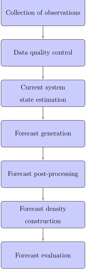
1.1 Schematic of a typical operational forecasting framework 19
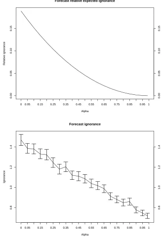
1.2 Skill of imperfect forecasts: the relative expected ignorance of the probabilistic binary forecasts drawn from the PDF p with respect to the true PDF q with increasing convergence α be-tween the two PDFs (top), and the empirical ignorance score of the probabilistic forecast Pi with respect to the true probability
Qi for a series of N = 211 binary outcomes with 95% likelihood
intervals (bottom). Forecast error results in larger values of rela-tive empirical ignorance compared to relarela-tive expected ignorance even where the forecast PDF is perfect (i.e. α= 1) . . . 33
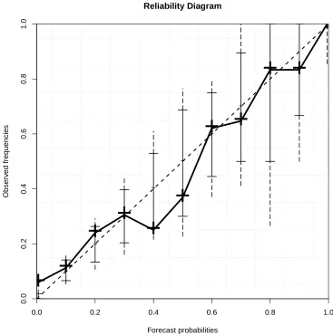
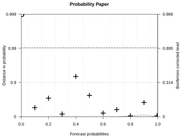
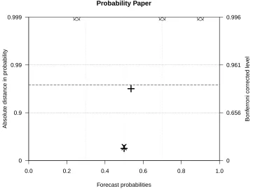
1.4 Forecast reliability on probability paper: an example of a reliability diagram on probability paper, corresponding to Fig.
1.3, showing that all but three forecast categories are consistent with forecast reliability. The dash–dotted line denotes the ex-act position of the diagonal. The right-hand axis indicates the equivalent Bonferroni corrected levels i.e. for a reliable forecast, all of the points (11 categories) would be expected to fall within the 0.99 probability distance band with an 88.6% chance. In ad-dition, the dashed lines indicate where the entire diagram would be expected to fall within with a 90% chance. The forecast prob-ability bin boundaries (grey dotted lines) have been determined by taking the mid-points between each probability category value. 38
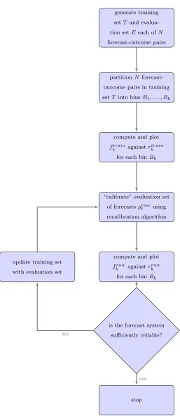
1.5 Schematic flowchart of forecast recalibration procedure. 43
1.6 Evolution of a forecast PDF: a schematic of a fan chart for a forecast PDF evolved in time. The right-hand axis labels the percentiles of the PDF. Darker shades represent more probable system states. The increase in spread is evident with time re-flecting the increase in uncertainty. This type of plot is used in several sections of thesis. . . 45
2.1 Ensemble forecasting under PMS:raw perfect Lorenz63 model ensemble generated in Expt. 1 (see table2.1) (top), and fan chart showing the kernel dressed ensemble (PDF) constructed from the raw ensemble shown in the upper plot at every time step from
t = 0 up tot=tτ = 6.4s(bottom). Each individual colour band
represents a 5% probability density percentile range of the PDF, from the 5th percentile to the 95th percentile (see Fig. 1.6for the fan chart key). In each plot, the true state of the system variable is shown as a blue trajectory, and the dashed horizontal lines denote the 50th, 90th, and 99th percentiles of the climatological distribution representing the thresholds θ ∈ {0.5,0.9,0.99}. The kernel dressed ensemble at time t =tτ = 6.4s would be blended
with the climatological distribution to produce the forecast PDF under the KDB method. . . 57
2.2 Ensemble forecasting under PMS: kernel dressed ensemble (PDF) corresponding to the PDF in Fig. 2.1 at t = tτ = 6.4s.
The true state of the system variable is shown as a blue line at ˜
xtτ = −5.7, and the dashed horizontal lines denote the 50th,
90th, and 99th percentiles of the climatological distribution rep-resenting the thresholdsθ∈ {0.5,0.9,0.99}. Given that ˜xtτ < xθ,
and that most of the probability density is below xθ = 0.37,
the forecast appears more skilful than a climatological forecast
pθ
clim = 0.5. . . 58
2.4 Forecast reliability on probability paper: reliability dia-gram on probability paper corresponding to Fig. 2.3. The two reliable forecast bins defined by [0.373,0.715] and [0.940,1.0] lie below the 0.9 probability distance dotted line. Circled symbols indicate an observed frequency outside the range of the y axis. The right-hand axis indicates the equivalent Bonferroni corrected levels for a reliable forecast so that the entire diagram (all 5 bins) would be expected to fall within the 0.99 probability distance band with an 95.1% chance. The dashed lines indicate where the entire diagram would be expected to fall within with a 90% chance if the forecast system was reliable. . . 60
2.5 Simple translation recalibration: reliability diagram schematic of thesimple translation recalibration algorithm using a training set of Lorenz63 binary forecast (asterisks) to recalibrate the eval-uation set of forecasts (pluses→crosses) both generated in Expt. 2 (see table 2.1). Most bins are translated closer to the diago-nal suggesting improved forecast reliability. Each bin is coloured differently for clarity. . . 65
2.6 Limitation of simple translation: distribution of forecastspre i
in the fifth binB5 (#{prei ∈B5}= 73) sorted in ascending order
2.7 Forecast recalibration using linear regression: Reliabil-ity diagram schematic demonstrating the linear regression recal-ibration algorithm using a training set of binned and averaged Lorenz63 binary forecasts (asterisks) to recalibrate the evaluation set of forecasts both generated in Expt. 2 (see table2.1). A linear regression line is fitted to the plotted points, from which the hor-izontal distance to the diagonal line determines the magnitude by which a raw forecast needs to be translated to be recalibrated. 69
2.8 Forecast recalibration using logistic regression: Reliability diagram schematic demonstrating the logistic regression recali-bration algorithm using a training set of binned Lorenz63 binary forecasts (asterisks) to recalibrate the evaluation set of forecasts both generated in Expt. 2 (see table 2.1). A logistic regression line is fitted to the plotted points, from which the horizontal dis-tance to the diagonal line determines the magnitude by which a raw forecast needs to be translated. For example, the two red lines show evaluation forecast probability values of 0.3 and 0.7 are calibrated to values of 0.16 and 0.89, respectively. Note that the fitted curve is a better fit than the linear regression line plotted in Fig. 2.7. . . 73
3.1 Ensemble forecasting under IMS: raw imperfect Lorenz63 model ensemble generated in Expt. 1 (see table 3.1) (top), and fan chart showing the kernel dressed ensembles (PDFs) constructed from the raw ensembles shown in the upper plot at every time step from t = 0 up to t = tτ = 6.4s (bottom). The PDF
repre-sents the probabilities of the system’s state and the blue trajec-tory shows the actual true state at a given time t. See Fig. 2.1
for further details. . . 91
3.2 Ensemble forecasting under IMS: kernel dressed ensemble (PDF) with Nens = 256 corresponding to that in Fig. 3.1 at
tτ = 6.4s. The true state of the system variable is shown as
a blue line at ˜xtτ = −5.7, and the dashed horizontal lines
de-note the 50th, 90th, and 99th percentiles of the climatologi-cal distribution representing the climatologiclimatologi-cal event thresholds
θ ∈ {0.5,0.9,0.99}. Given that ˜xtτ < xθ, and most of the
proba-bility density is below xθ = 0.37, the forecast is more skilful than
a climatological forecast pθ
clim = 0.5, although not as skilful as
the perfect model forecast in the equivalent plot in Fig. 2.2. . . 92
3.3 Forecast ignorance under IMS: ignorance (with 5% - 95% uncertainty intervals) for binary forecasts produced from the NC (solid line), AC (dashed line), Bayesian (dotted line), and KDB (dash-dotted line) density construction methods under Expt. 2 (see table 3.1) with θ = 0.9, τ = 25.6s and all ensemble sizes. The KDB method performs best at smaller ensemble sizes, and is equalled in skill for ensemble sizes Nens≥128 by the NC and
AC methods. Note: there is no curve for the NC method where
Nens<128 because it produces forecast busts at these ensemble
3.4 Forecast reliability after recalibration: An example relia-bility diagram showing the changes in reliarelia-bility of the raw set (crosses) and recalibrated evaluation set (pluses) of AC forecasts using the simple translation algorithm. The recalibrated fore-casts appear to be more reliable than the raw forefore-casts; this is supported by the numerical values of the reliability component of ignorance before and after recalibration are IGNREL = 0.178
and IGNREL = 0.007. All sets of forecast-outcome pairs are
generated under Expt. 3 (see table 3.1) . . . 102
3.5 Forecast reliability after recalibration: Reliability diagram on probability paper showing the changes in reliability of the raw set (crosses) and recalibrated evaluation set (pluses) of AC fore-casts using the simple translation a with 5% - 95% (1% - 99% vertical dashed line) consistency bars. The recalibrated forecasts are clearly more reliable than the raw forecasts. Only one out of four raw forecast bins falls within the Bonferroni corrected 0.99 probability distance (upper dotted) band, indicating an unreli-able forecast before recalibration. All sets of forecast-outcome pairs are generated under Expt. 3 (see table 3.1). . . 103
3.6 Forecast binning: Reliability diagram showing the variation in sampling error where the forecast bins are not equi-probable. The bin with boundaries [5.8×10−13,1.0] has a bin population
of 16 whereas the bin with boundaries [0,5.8×10−13] has a bin population of 496. The calibration function estimate ˆκ(r2) has
3.7 Forecast reliability after recalibration: reliability diagram showing the forecast reliability of the raw set (crosses) and recali-brated evaluation set (pluses) using the KDE algorithm. The po-sition of the raw and recalibrated forecast bins suggests that the recalibrated forecasts are more reliable than the raw forecasts and the changes to forecast skill and reliability (i.e. ∆IGN =−0.187 and ∆IGNREL = −0.172, respectively) confirm the
improve-ment. All sets are generated under Expt. 3 (see table 3.1). . . . 111
3.8 Forecast reliability after recalibration: reliability diagram on probability paper showing the forecast reliability of the raw set (crosses) and recalibrated evaluation set (pluses) using the KDE algorithm with 5% - 95% (1% - 99% vertical dashed line) consistency bars.The improvement in reliability is more evident since both the recalibrated forecast bins lie within the Bonferroni corrected 0.99 probability distance (upper dotted) band whereas only one raw forecast bins does so. All sets are generated under Expt. 3 (see table 3.1). All other details are identical to Fig. 3.5. 112
3.10 Forecast reliability after recalibration: Reliability diagram on probability paper showing KDB forecast reliability of the raw set (crosses) and recalibrated evaluation set (pluses) using the simple translation method with 5% - 95% (1% - 99% vertical dashed line) consistency bars. The right-hand axis indicates the equivalent Bonferroni corrected levels e.g. for a reliable forecast, all of the points (7 bins) would be expected to fall within the 0.99 probability distance band with a 93.2% chance. In addition, the dashed lines indicate where the entire diagram would be expected to fall within with a 90% chance. Recalibration is ineffective here since the forecasts are already well-calibrated. All sets are generated under Expt. 5 (see table 3.1). . . 114
3.11 Simple translation recalibration: reliability diagram schematic of thesimple translationrecalibration method using a training set of Lorenz63 binary forecasts (asterisks) to recalibrate the evalu-ation set of forecasts (pluses → crosses) both generated in Expt. 6 (see table 3.1). Recalibration has resulted in most bins being translated closer to the diagonal so that forecast resolution is decreased. Raw resolution was already low in this case so the de-crease is relatively small ∆IGNREL =−0.003, but this example
4.1 Serial correlation in forecast skill statistics: time series of 27 IGN scores of forecasts of Lorenz63 system states (top)
and bootstrap resamples of the same time series (bottom). The time series is serially correlated while the bootstrap resamples are serially independent. Averages over sequential samples of size
N = 16 (red lines) tend to deviate from the IGN estimate over the entire time series (IGN =−5.05; horizontal line) in the top plot compared to the bottom plot, resulting in a sampling distribution of the averages which is larger. The sampling variances of the 8 subsamples are s2
IGN = 0.15 ands2IGNboot = 0.06. . . 124
4.2 LCBR model forecast skill statistics under serial depen-dence: sampling variances of IGN estimates computed from
N = 210 simulations correlated time series (r
1(y) ≈ 0.8; red
circles) of reliable forecasts (a = 0, b = 1) of a low probability event (µy = 0.05) and bootstrap resamples (r1(y)≈ 0; blue
4.3 Statistical inference of LCBR model forecast skill under serial dependence: probability coverage of 95% confidence in-tervals forN = 210IGN estimates computed from a serially
corre-lated time series (r1(y)≈0.8) of reliable forecasts (a= 0, b= 1)
of a low probability event (µy = 0.05) and bootstrap resamples
(r1(y)≈0; blue circles), both shown with increasing sample size.
The plot demonstrates that confidence intervals are too compact under serial dependence by showing that the probability cover-age of the confidence intervals for the serially correlated IGN statistics is lower than those for the non-serially correlated IGN statistics. As N increases, the probability coverages of both con-verge onto the nominal 95% coverage (dashed line) but a larger sample size is required for the former to do so. The values of lag-1 autocorrelation, climatological probability, and model pa-rameters are identical to Fig. 4.2. . . 134
4.4 Statistical inference of LCBR model forecast skill un-der serial dependence: IGN estimates of correlated time se-ries plotted against 95% confidence interval widths computed from the IGN statistics of a correlated time series (r1(y)≈ 0.8)
of reliable forecasts (a = 0, b = 1) of a low probability event (µy = 0.05). The plot shows how confidence intervals tend to
be too narrow under serial dependence where forecasts are more skilful and where sample sizes are too small. The values of lag-1 autocorrelation, climatological probability, and model parame-ters are identical to Fig. 4.2. . . 135
4.5 Lorenz63 observations: time series of x state variable obser-vations illustrating the bimodal behaviour of the Lorenz63 at-tractor. The observations have a strong degree of linear serial correlation (r1(y) ≈ 0.96) measured over the whole sample size
4.6 Lorenz63 forecast skill statistics under serial dependence: Sampling variances of a) ignorance estimates computed from forecasts of a correlated time series of Lorenz63 observations (r1(y) ≈ 0.94; red circles) and b) the natural measure of
ig-norance estimates (r1(y)≈0; blue circles), both with 5%−95%
uncertainty intervals. There is a clear inflation of the sampling variances until at least a sample size of 25 showing that the serial
correlation in the observations is transmitted to the score statistics.138
4.7 Statistical inference of Lorenz63 forecast skill under se-rial dependence: probability coverage of 95% confidence inter-vals for increasing sample size (top), and IGN estimates of cor-related Lorenz63 forecast time series plotted against 95% confi-dence interval widths (bottom). The two plots show the tendency of confidence intervals to be too compact under serial dependence where forecasts are more skilful or sample sizes are too small. . . 139
4.8 AR(1) forecast skill statistics under serial dependence: Estimates of sampling variances of IGN estimates for an AR(1) observation time series (ϕ = 0.9; red circles) and the boot-strapped observations (blue circles). Both sets of points all lie within 95% uncertainty intervals constructed from Nboot = 27
bootstrap resample estimates of the sampling variance of Gaus-sian distributed forecasts showing that there is no significant dif-ference between either of the sampling variances and uncorrelated Gaussian forecasts. Each sampling variance estimate contains 28
4.9 AR(1) forecast skill statistics under serial dependence: Example of a 1 step delay plot showing the lack of linear serial correlation in a single IGN time series of sample size N = 210
computed from serially correlated observations (ϕ = 0.9). The red coloured points, denoting ignorances scores −log(p(st+1))>
3 (signifying less skilful forecasts) at time t + 1 (y-axis), also indicate that forecasts are more skilful at timet, highlighting the lack of serial correlation. The mean and standard error of the lag-1 autocorrelation values of theNboot = 28 replications of time
series are not significantly different from zero. . . 143
4.10 AR(1) forecast skill statistics under serial dependence: Mean sampling variance of the IGN for AR(1) time series of fore-casts of serially correlated observations (r1(y) = 0.9; red line),
forecasts of bootstrapped observations (r1(y) ≈ 0; blue line),
and climatological forecasts (green line), all with 5%−95% un-certainty intervals computed from Nboot = 27 samples. There is
a clear inflation of the climatological sampling variance . . . 144
4.11 Hurricane forecast forecast skill statistics under serial dependence: Sampling variances of IGN estimates computed for 28 time series of serially correlated observations (r
1(y)≈0.4;
red line) and bootstrapped observations (r1(y)≈0; blue line). . 147
4.12 Logistic map: the logistic map given by xi+1 = 4xi(1−xi).
The parabolic shape of the curve indicates the presence of serial dependence although there is zero lag-1 autocorrelation (r1(y)∼
4.13 Logistic map forecast skill: theoretical ignorance expected (relative to T IE with σtruth = 1/128) at f(f(x)) and f(x) of a
single logistic map time series (α = 4.0) of sample size N = 28.
A linear fit is shown as a dashed line and the value of the lag-1 ACF of the time series is r1(T IE) = −0.26, both indicating a
degree of negative linear serial correlation in the skill score time series. . . 151
4.14 Logistic map forecast evaluation statistics under serial dependence: sampling variances of a)T IEestimates computed from forecasts of a correlated time series of Logistic map ob-servations (r1(T IE) ≈ −0.26; red line) and b) T IE estimates
(r1(T IE)≈0; blue line) computed from forecasts of the natural
measure of the Logistic map, both with 5%−95% uncertainty intervals. There is a clear deflation of the sampling variances of a) until at least a time window length of 25 showing that the
serial correlation in the observations is transmitted to the score statistics. . . 152
4.15 Information deficit time series: 29 step time series of
infor-mation deficit statistics for Lorenz63 forecasts constructed us-ing IN (blue line) and PDA (red line) data assimilation schemes (τ = 0.1). The PDA forecasts are have a lower information deficit
IDP DA = 0.18 bits compared to the IN forecasts IDIN = 0.21
bits over this time window. The differences between the informa-tion deficit values for the two forecast systems tend to be smaller than the corresponding differences in IGN, the values of which are IGNP DA = −5.30 and IGNIN = −3.57 for the same
4.16 Sampling variance with IN and PDA: Sampling variances of ID estimates computed from IN (top) and PDA (bottom) forecasts (∆ = 0.1, τ = 0.1) of a) a correlated time series of Lorenz63 observations (red circles) and b) the natural measure of ID estimates (blue circles) with increasing sample size, both with 5%−95% uncertainty intervals. . . 157
4.17 Forecast skill with PDA: forecast ID (∆ = 0.1, τ = 0.1) il-lustrating the degree of predictability of the Lorenz63 system in state space. The double fixed point attractors are clearly repre-sented by the ID samples in state space. Black circles denote very skilful forecasts (ID <−2) while black squares denote very poor forecasts (ID >4). . . 159
5.1 Distribution of insured losses caused by U.S. natural catastrophes 1950-2011: the distribution of insured losses (normalised to 2011 dollars for inflation) incurred by the insur-ance industry due to U.S. natural catastrophes during 1950-2011. Tropical cyclones have caused 63% of the total insured losses. Data source: TOPICS GEO 2011, Munich Re . . . 169
5.3 Empirical skill of SC forecasts: the distribution of the em-pirical relative ignorance of 2048 clients’ forecasts when betting against cooperative insurer’s climatological forecasts from 1966-2012 with parameters δ= 1 andǫ= 1. The median is constantly negative indicating that the skill of the majority of clients’ fore-casts is greater than the cooperative insurer. . . 180
5.4 Client’s accumulation of wealth: the distribution of clients’ profit ct− c0 in rounds of Hurricane Roulette over the period
1966-2012 computed from 211 simulations. 90% of clients have
profited within 50 years by betting on the synoptic conditioning forecast system against the cooperative insurer’s climatological forecast. . . 181
5.5 Client’s wealth: The distribution of clients’ return ratios u in rounds of Hurricane Roulette over the period 1966-2012 com-puted from 211 simulations. The median lies above the u = 1
line indicating that most clients have profited by betting on the synoptic conditioning forecast system against the cooperative in-surer’s climatological forecast. Also given the log scale, the av-erage (arithmetic mean) wealth of a punter is well above zero (i.e. the house has also lost). The bumps reflect where forecast PDFs are sharper (i.e. El Ni˜no phases where the Poisson mean parameter λA is smaller) resulting in more extreme incidences of
forecast skill. . . 182
5.7 Statistical inference of U.S. landfall fractions: 95% score confidence intervals computed from 1966-2012 U.S. landfall frac-tion rate. ‘+’ symbols correspond to the fracfrac-tions for each land-fall count category. . . 187
5.8 Atlantic basin hurricane counts: Example 50 year time series of synthetic CAT1-5 Atlantic basin hurricane counts. The mean (dashed line) corresponds to the real-world dataset average, and the solids line represents the 5-year running mean. . . 199
5.9 Forecast skill of CA forecasts: Ignorance scores computed for three training sets of single (red lines line) and series (blue lines) analogue forecasts at increasing window lengths. The score minima are shown for both the single (plus) and series analogue methods (cross). The single and series analogue methods both demonstrate skill relative to climatology, and better than the Bayesian forecast (green line), but are outperformed by the per-fect model forecast (brown line). . . 200
5.10 System, forecast, and climatology: probability distributions for the system (black), and an imperfect model (green) for phase year φ = 12 of the 24 year cycle. The climatological PDF (com-puted over all values of φ) is also shown in blue. The imperfect model PDF appears is a better fit than the climatological PDF with respect to the difference between the expected ignorance of the two (i.e. E[IGNf cst]−E[IGNclim] =−0.11). . . 203
5.11 Time to forecast skill: Distribution of forecast skill p-values (H1 : IGN < 0) of 211 independent statisticians (simulations)
5.12 Time to forecast value: Percentage of 211 independent
under-writers expected to make a profit with time when betting against climatology using the imperfect model in a game of hurricane roulette (main plot), and frequency distribution of underwriters’ wealth with time (inset plot). 99% of underwriters make a profit by 35 years, much earlier than the time for 99% of the statisti-cians to prove the skill of the forecast system (> 100 years for
IGN). . . 208
5.13 Bettor’s wealth: Scatter plot of wealth vs ignorance (top) and wealth vs forecast mean-verification correlations (bottom) for 211 underwriters who bet using the imperfect hurricane
fore-cast model over different time windows. The vertical dotted line shows the threshold of relative skill (better than climatology) while the horizontal dotted line indicates the profit line. The re-lationship between IGN and wealth is strictly monotonic while the relationship between linear correlation r and wealth is not, highlighting the importance of employing proper scoring rules. NB: the x-axis in the top plot is negatively orientated. . . 210
6.2 NHC 2012 TC forecast reliability: reliability diagram for the NHC’s 2012 48-hr TC forecasts* with 5% - 95% (1% - 99% vertical dashed line) consistency bars. All but three forecast cate-gories lie within the consistency bars, indicating that the forecast system is mostly reliable. The forecast probability bin bound-aries (grey dotted lines) have been determined by taking the mid-points between each probability category value. *Sourced from NHC online Tropical Weather Outlooks. . . 220
6.3 NHC 2012 TC forecast reliability: reliability diagram on probability paper for the NHC’s 2012 48-hr TC forecasts* show-ing that all but three forecast categories are consistent with fore-cast reliability. The dash–dotted line denotes the exact position of the diagonal. The right-hand axis indicates the equivalent Bonferroni corrected levels i.e. for a reliable forecast, all of the points (12 categories) would be expected to fall within the 0.99 probability distance band with an 88.6% chance. In addition, the dashed lines indicate where the entire diagram would be ex-pected to fall within with a 90% chance. The forecast probabil-ity bin boundaries (grey dotted lines) have been determined by taking the mid-points between each probability category value. *Sourced from NHC online Tropical Weather Outlooks. . . 221
6.5 Recalibrated NHC 2012 TC forecast reliability: reliabil-ity diagram for the NHC 2012 TC forecasts recalibrated using 2011 forecasts as training set with 5% - 95% (1% - 99% vertical dashed line) consistency bars. Forecast recalibration has resulted in a decrease of forecast reliability since most recalibrated prob-ability categories (pluses) have larger probprob-ability distances than raw forecast categories (crosses). For a reliable forecast, all of the points (8 categories) would be expected to fall within the 0.99 probability distance band with an 92.3% chance. The forecast probability bin boundaries (grey dotted lines) are identical to those on the original 2012 reliability diagram although the num-ber of populated categories has decreased to 8. Refer to Fig. 6.3
for further details. *Sourced from NHC online Tropical Weather Outlooks. . . 225
6.7 Recalibrated NHC 2012 TC forecast reliability: reliability diagram for the NHC 2012 TC forecasts recalibrated using leave-one-out cross-validation with 5% - 95% (1% - 99% vertical dashed line) consistency bars. Seven of the nine recalibrated probability categories (pluses) have smaller probability distances than raw forecast categories (crosses). The reliability curve shows that leave-one-out recalibration can both significantly improve and decrease reliability depending on the categorisation of the fore-casts. All of the points (9 categories) would be expected to fall within the 0.99 probability distance band with an 91.4% chance. The forecast bin boundaries (grey dotted lines) are identical to those on the original 2012 reliability diagram. Refer to Fig. 6.3
for further details. *Sourced from NHC online Tropical Weather Outlooks. . . 229
6.9 NHC 2012 TC forecast Time Until Event: CDFs of NHC 2012 TC forecast* TUE times (in hours) for each forecast prob-ability category rk (solid lines), and for a set of reliable forecasts
(fk=rk) where the TUE times are computed with a discrete
uni-form distribution function (dashed lines). The higher probability curves lie well above the corresponding uniform distribution of reliable forecast TUE lengths. The TUE categories indicate the occurrence of a TC event between the time given and 6 hours pre-vious to it, and “NO” indicates a non-occurrence of a TC within 48 hours. *Sourced from NHC online Tropical Weather Outlooks. 231
6.10 NHC 2012 TC forecast Time Until Event: Maximum, min-imum (minuses) and median (pluses) of verifying NHC 2012 TC forecast* TUEs for each forecast probability category, rk. The
TUE time categories indicate the occurrence of a TC event be-tween the time given and 6 hours previous to it. *Sourced from NHC online Tropical Weather Outlooks. . . 232
7.1 Time series of all annual Atlantic basin named storm counts from 1966-2012 with CAT1-5 basin hurricanes and CAT1-5 U.S. Land-falls shown as sub-categories (top), and CAT1-5 basin hurricanes and CAT3-5 Basin hurricanes shown as sub-categories (bottom). 242
7.2 Modelling Atlantic basin CAT1-5 basin hurricanes: fit-ted values of the rate of CAT1-5 Atlantic basin hurricane annual counts µ regressed on SSTAtl and SSTtrop from 1966-2012 with
linear (green line), quadratic polynomial (dark blue), and cubic spline (light blue) Poisson regression models. The linear fit cor-responds to the best-fit model in the second column of Table 7.1
8.1 Synoptic conditioning forecast for 2013: SC forecast (red) and climatological forecast (blue) PDFs for Atlantic basin named storms in 2013. The synoptic conditioning technique utilises in-formation on the annual August-October ENSO phases. There were 13 named storms in 2013 (axis label coloured red) which the SC forecast PDF has assigned larger probability mass to than the climatological PDF, and hence, has achieved superior skill
IGN =−0.28. . . 268
8.2 Conditional analogue forecast for 2013: single CA fore-cast (red) and climatological forefore-cast (blue) PDFs for Atlantic basin named storms in 2013. There were 13 named storms in 2013 (axis label coloured red) which the CA forecast has as-signed larger probability mass to than the climatological PDF, and hence, achieves superior skill IGN =−0.40. . . 270
8.3 Poisson GLM forecast for 2013: Poisson GLM forecast (red) and climatological forecast (blue) PDFs for Atlantic basin named storms in 2013. The regression coefficients of the model are:
β0 = 2.01, β1 = 0.01 (year), β2 = 0.97 (SSTAtl), and β3 =−1.37
(SSTtrop). There were 13 named storms in 2013 (axis label
8.4 NHC 2013 TC forecast reliability: reliability diagram for the NHC’s 2013 48-hr TC forecasts* with 5% - 95% (1% - 99% vertical dashed line) consistency bars. Forecast categories 80% and 90% have consistency bars with wide intervals and medians which lie off the diagonal because of small bin populations. The forecast probability bin boundaries (grey dotted lines) have been determined by taking the mid-points between each probability category value. *Sourced from NHC online Tropical Weather Outlooks. . . 276
8.6 Recalibrated NHC 2013 TC forecast reliability: reliabil-ity diagram for the recalibrated NHC 2013 TC forecasts using 2012 forecast-outcome set as training data with 5% - 95% (1% - 99% vertical dashed line) consistency bars (the highest cate-gory r7 = 0.999 has a consistency bar with zero width). The
forecast probability bin boundaries (grey dotted lines) are iden-tical to those on the original 2013 reliability diagram although the number of populated categories has decreased to 7. Forecast recalibration has resulted in a decrease of forecast reliability (c.f. Fig. 8.4). *Sourced from NHC online Tropical Weather Outlooks. 279
8.7 Recalibrated NHC 2013 TC forecast reliability: reliability diagram for the NHC 2013 TC forecasts recalibrated using the 2011 forecast-outcome set as training data with 5% - 95% (1% - 99% vertical dashed line) consistency bars. Forecast recalibra-tion has resulted in a decrease of forecast reliability since most recalibrated probability categories (pluses) have larger probabil-ity distances than raw forecast categories (crosses). The forecast probability bin boundaries (grey dotted lines) are identical to those on the original 2013 reliability diagram although the num-ber of populated categories has decreased to 7. See Fig. 8.5
8.8 NHC 2013 TC forecast Time Until Event: fractions of ver-ifying NHC 2013 TC forecasts* having different TUE lengths (in hours) for all probability categories. The coloured TUE cate-gories denote the occurrence of TC formation between the time given and 6 hours previous to it. There is a clear pattern of larger fractions of shorter TUE with increasing forecast probability cat-egory. Total counts of verifying forecasts for each category are shown at the top of the bars. *Sourced from NHC online Tropical Weather Outlooks. . . 281
8.9 NHC 2013 TC forecast Time Until Event: CDFs of NHC 2013 TC forecast* TUE times (in hours) for each forecast prob-ability category rk (solid lines), and for a set of reliable forecasts
(fk=rk) where the TUE times are computed with a discrete
uni-form distribution function (dashed lines). The higher probability curves lie well above the corresponding uniform distribution of reliable forecast TUE lengths. The TUE categories indicate the occurrence of a TC event between the time given and 6 hours previous to it, and an “NO” indicates a non-occurrence of a TC within 48 hours. *Sourced from NHC online Tropical Weather Outlooks. . . 282
C.1 Diagnostics plots and worm plot for Poisson model of Atlantic basin named storm counts regressed on year, SSTAtl and SSTtrop
from 1966-2012. . . 302
C.2 Diagnostics plots and worm plot for Poisson model of Atlantic basin CAT1-5 hurricane counts regressed on SSTAtl and SSTtrop
from 1966-2012. . . 303
C.3 Diagnostics plots and worm plot for Poisson model of Atlantic basin CAT3-5 hurricane counts regressed on SSTAtl and SSTtrop
C.4 Diagnostics plots and worm plot for Poisson model of Atlantic CAT1-5 US landfall counts regressed on SSTAtl and SSTtrop from
1966-2012. . . 305
C.5 Diagnostics plots and worm plot for logistic model of Atlantic basin CAT3-5 hurricane count fractions regressed on year from 1966-2012. . . 306
C.6 Diagnostics plots and worm plot for logistic model of Atlantic CAT1-5 US landfall count fractions regressed on SSTAtl from
2.1 Configurations for PMS Lorenz63 binary forecast exper-iments . . . 54
2.2 Forecast skill before and after recalibration under PMS 84
3.1 Configurations for IMS Lorenz63 binary forecast exper-iments . . . 93
3.2 Forecast skill before and after recalibration under IMS . 99
3.3 Reliability diagram bin specification methods . . . 106
3.4 Forecast skill before and after recalibration . . . 109
4.1 Experimental Configurations for Lorenz63 Forecasts . . 156
5.1 Single and series analogue methods for forecast of the 1990 hurricane season . . . 192
5.2 Hypothesis tests of forecast skill . . . 207
6.1 NHC 2012 TC forecast reliability diagram statistics . . . 223
6.2 NHC 2012 TC forecast reliability diagram statistics by TUE . . . 233
7.1 Poisson regression models of Atlantic basin storms 1966-2012 . . 258
7.2 Logistic regression models of Atlantic basin storms 1966-2012 . . 261
8.1 2013 hurricane forecast skill (IGN) . . . 273
8.3 NHC 2012 TC forecast reliability diagram statistics by TUE . . . 283
Forecast evaluation and recalibration with dynamical systems
α Blending Parameter . . . .46
κ(·) calibration function . . . .61
IGN ignorance . . . .79
N sample size . . . .53
Nens ensemble size . . . .53
p(·) probabilistic forecast density . . . .26
pclim(·) climatological probability density . . . .25
st observed state of a system . . . .23
S forecast scoring rule . . . .28
t time . . . .24
θ climatological distribution quantile . . . .53
τ forecast lead time . . . .53
xt observation of state variable x at timet . . . .53
˜
xt true state of system variable variable x at timet . . . .52
xθ climatological distribution quantile of state variable x . . . .53
Ψ fixed rule of a dynamical system . . . .13
y outcome . . . .44
Forecast evaluation under serial dependence
α beta distribution parameter . . . .131
αblend blending parameter . . . .156
β Beta distribution parameter . . . .131
BS Brier . . . .132
Γ gamma function . . . .131
∆ forecast launch step . . . .156
IGN ignorance . . . .128
N sample size . . . .129
N′ effective sample size . . . .132
Nboot number of bootstrap resamples . . . .142
p(·) probabilistic forecast density . . . .128
pclim(·) climatological probability density . . . .154
ρ forecast PDF . . . .149
φ phase constant . . . .146
Φ standard Normal distribution CDF . . . .131
ϕ model lag-1 autocorrelation parameter . . . .131
r1 lag-1 autocorrelation . . . .132
t time . . . .138
τ forecast lead time . . . .137
y outcome . . . .129
z Gaussian variate . . . .131
Hurricane modelling and forecasting
α B-spline function coefficient . . . .247
B piecewise cubic B-spline basis function . . . .247
c betting client’s capital . . . .180
n number of annual hurricanes . . . .185
N sample size . . . .176
f(·) GAM basis function . . . .243
g(·) link function . . . .243
G(·) growth function . . . .183
η linear predictor . . . .243
p(·) probabilistic forecast of a hurricane outcome . . . .177
pclim(·) unconditional climatological PDF . . . .175
π binomial distribution parameter . . . .245
φ phase constant . . . .176
q(·) true probability distribution of hurricane outcome . . . .200
r Pearson correlation coefficient . . . .205
Tp period of testbed hurricane system . . . .198
u return ratio . . . .182
x regression model predictor variable . . . .243
yc testbed hurricane system y-offset . . . .198
Introduction
Since the pioneering of modern-day weather forecasting by Robert Fitzroy in 1861 [138], the accuracy and efficiency of predictions of weather including ex-treme events such as tropical storms have progressed significantly. Probabilis-tic forecasting, in parProbabilis-ticular, has emerged as an essential tool in operational weather forecasting since the U.S. Weather Bureau began issuing subjective probabilistic forecasts of precipitation in 1965 [141]. Indeed, understanding and quantifying uncertainties about the future evolution of a complex system such as the Earth’s ocean-atmosphere system is best addressed using the probabilis-tic approach. Probabilisprobabilis-tic forecasts contrast with point forecasts which only provide a single value prediction of an outcome, and hence do not commu-nicate uncertainty. Furthermore, reliable probabilistic forecast information is generally more informative for forecast users, allowing them to optimise their decision-making [191].
potential value for insurance, policy-making, and civil planning [43, 117, 156]. Operating within a robust statistical framework for best-practice forecasting is therefore important to maximise the benefit of predictive information.
This chapter is structured as follows: the fundamental topics of probabilistic forecasting and Atlantic basin hurricanes are briefly introduced in Sections 1.1
and 1.2, followed by an overview of this thesis in Section 1.3.
Sections 1.4 to 1.9 provide background on many of the theoretical conven-tions, terminology, and notation covered in this thesis, allowing later chapters to focus on what is new. Other than the presentation itself, there is little new material in this chapter.
The sections in this chapter are summarised as follows: a review of some ba-sic concepts of forecasting, a fundamental topic of this thesis, is given in Section
1.1
Probabilistic forecast framework
Probabilistic forecasts are typically constructed from a collection, or ensem-ble, of point forecasts produced from dynamical model output (e.g. numerical weather models [114]), but can also be constructed using statistical models based on past observational data [200], or even from a hybrid of the two [205]. Whichever method is employed, either a finite set of probabilities of discrete outcomes or a probability density function for continuous outcomes is usually the resulting output information. These probability distributions express the uncertainty in the forecasts, reflecting the predictability of the future evolution of a system.
There are difficulties which are unique to probabilistic forecasts, however, in part because more sophisticated methods are necessary to produce probabilistic information, and also because they are perceived to be more challenging to com-municate than point forecasts. There are, in fact, a number of stages typically involved in the process of operational forecasting, whether probabilistic or not. These are listed in a typical chronological order as:
1. data retrieval and transformation;
2. current system state estimation;
3. ensemble construction;
4. ensemble post-processing;
5. forecast evaluation.
Forecast evaluation
Forecast evaluation plays a critical role not only in monitoring forecast qual-ity, but also in increasing the effectiveness of predictive weather information for decision-making support. The evaluation stage includes the collection of
forecast-outcome pairs; consisting of a single forecast of a given outcome in the future and the actual outcome observed. The performance of single forecast is assessed by assigning it a value according to a numerical performance mea-sure which is a mathematical function of the forecasts and the outcomes. The purpose of the performance measure is to determine the degree of “correspon-dence” between the forecasts and outcomes. A common type of performance measure is called a scoring rule [60, 87], which is defined for individual pairs of forecasts and outcomes, and quantifies forecast accuracy, or “skill”. An example of a scoring rule for point forecasts is Root Mean Square Error (RMSE) [136]. RMSE is a measure of the “distance” between a forecast and the correspond-ing outcome. While this is an intuitively appealcorrespond-ing measure of performance, it is doubtful whether the true quality of a point forecast can be expressed with RMSE. The problem is that the point forecast and RMSE only hold information about the statistical expectations of the forecasts and forecast performance. An important requirement of measuring the performance of a forecast is that the information contained in the full joint distribution of forecasts and outcomes is included in the measurement [142]. This is the basis for robust forecast evalua-tion, and is a guiding principle behind the best-practice evaluation techniques discussed in this thesis.
data can be replicated in the forecasts, and hence, the performance measure statistics. Consequently, the variances of the sampling distributions of the per-formance measure can become “inflated”, resulting in erroneous estimates of forecast skill.
Forecast recalibration
During the post-processing stage of the forecasting process, statistical meth-ods are commonly employed to improve the quality of forecasts that contain systematic (i.e. persistent) errors. Typically, a procedure called calibration is performed where biases in the mean and variance of forecast probability distri-butions are corrected by simply adding or multiplying by constants. A superior approach which utilises the joint forecast-outcome distribution (i.e. measures forecast skill) by, for example, using a linear regression to model past sets of forecasts on their corresponding outcomes, is recalibration. Recalibration can be used to improve a particular attribute of forecast performance called relia-bility. Specifically, reliability is a measure of the statistical consistency between the forecasts and the conditional expectations of the outcomes given a forecast probability. In short, it measures the “closeness” between forecast probability values and the observed relative frequency of an outcome. Forecast reliability is generally improved using recalibration where models suffer from systematic bias, making it a useful and relatively straightforward technique in the fore-cast post-processing stage. A number of statistical techniques are employed in this thesis to assess the effectiveness of recalibration when applied to forecast models.
1.2
Hurricane forecasting
to understand the physical mechanisms of hurricanes and improve predictions of hurricane activity on various timescales [64, 50, 28, 181]. Forecast informa-tion can potentially be of significant value to policy-makers, the commercial and insurance sectors, and for the general public [43]. Skilful predictions of coastal hurricane strikes on annual to decadal timescales are of huge potential value for applications such as land use planning, hazard mitigation, emergency management, and (re)insurance pricing [149]. There is a large degree of uncer-tainty in hurricane predictions on climatic timescales [164], however, and the out-of-sample skill of seasonal (i.e. up to a year ahead) forecasts is still yet to be proven [46,156]. These limitations are due to the inadequacy of numerical mod-els for simulating the climate system, and the relatively short length of a reliable historical hurricane data archive [106]. In this thesis, a number of novel and easily deployable statistical forecast systems are presented for constructing pre-dictions of seasonal hurricane counts (i.e. annual numbers of hurricanes). While these forecast systems are potentially skilful, the key purpose is to demonstrate robust practice in statistical forecast construction and forecast evaluation.
activity in this thesis.
1.3
Thesis overview
The structure of this thesis is outlined as follows:
The effectiveness of forecast recalibration is investigated under perfect and imperfect model scenarios in Chapters2and3in the context of a well known dy-namical system called Lorenz63 [118]. The performance of binary forecasts (i.e. forecasts of an event with two possible outcomes) of the state of the Lorenz63 system is compared before and after recalibration. These forecasts have been constructed with different forecast density construction methods which are also defined. The results of the recalibration experiments using a number of re-calibration algorithms sourced from the literature are presented. Information-theoretical measures of forecast performance are defined, and are used to assess any improvements in forecast skill, forecast reliability, and forecast resolution. It is shown that recalibration is most effective where forecast performance is already poor. The investigation of recalibration comprises a new contribution in this thesis. The concept of “optimal skill” for binary forecasts, an upper bound on forecast skill for a particular performance measure, is also introduced for the first time.
esti-mates of forecast skill to be inaccurate. A new empirical method for sample size corrections is also proposed.
Chapters 6, 7, and 5 review and extend the current methodology for hur-ricane modelling and prediction, and provide insights into best practice when evaluating and utilising hurricane forecasts.
In Chapter 6, a case-study of forecast recalibration is applied to short-term (i.e. 48-hour ahead) forecasts of tropical cyclone formation issued by the Na-tional Hurricane Center based in the U.S.. Recalibration is performed both out-of-sample and with leave-one-out cross-validation to assess whether the per-formance of the tropical cyclone forecasts can be improved. While the latter technique increased the reliability of the forecasts, the out-of-sample approach generally led to a deterioration of reliability. This is explained by year-to-year variability in patterns of hurricane formation. It is also shown that the as-sessment of the reliability of these forecasts is complicated by variation in the time between forecast issuance and the occurrence of tropical cyclone formation, referred to as “Time Until Event”.
In Chapter 7, Poisson and logistic regressions are used to model annual counts of various categories of hurricanes, and fractions of subset categories of hurricanes using a variety of predictor variables. Various techniques are employed to fit and select the models so that nonlinear dependencies between the response variable (i.e. hurricane variable) and the predictors, as well as collinearity between predictors, are accounted for. An innovative computational “sliding linear” root-finding algorithm for constructing confidence intervals for regression coefficients where sample sizes are small is presented for the first time.
analogue” are introduced. These techniques have been designed to exploit the data available in the relatively short hurricane data archive. The limitations of statistical inference with small samples of small-number count data are also discussed, followed by suggested methods which are specialised for these types of data. In addition, the relationship between forecast skill and forecast value is examined in a monetary betting scenario to demonstrate that a forecast user need not wait to establish statistical confidence in the skill of a forecast system before putting it to use. This concept is aptly titled “profit before proof”.
Finally, the forecast systems based on the techniques discussed in Chapters7
and5are fitted to the historical hurricane dataset, and are deployed in Chapter
8to construct a real-time outlook for the 2013 Atlantic basin hurricane season. The skill of these forecasts is evaluated and compared to other operational predictions.
The key new contributions and innovations in this thesis are summarised as follows:
1. critique of existing recalibration algorithms for binary probabilistic fore-cast recalibration. Kernel density estimation [23] and beta-transform lin-ear pool [165] algorithms are shown to perform the best out of all the algorithms.
2. examination of the relationship between forecast skill and forecast reliabil-ity in the context of recalibration using the decomposition of the ignorance score
3. surveyance of the conditions where recalibration is effective for increasing forecast reliability and forecast skill
4. introduction, discussion and quantification of “optimal skill” of binary forecasts
recalibration, and review and critique of binning/categorisation methods in the literature
6. identification of the conditions where recalibration has a detrimental effect on forecast resolution
7. derivation of the analytical sampling variance of ignorance score estimates for binary forecasts
8. demonstration of how misleading estimates of forecast skill can result from the presence of serial correlation in evaluation data (with both a stochastic and nonlinear dynamical system)
9. explanation of how the presence of serial correlation in evaluation data is neither a necessary nor sufficient condition for misleading estimates of forecast skill (with stochastic systems)
10. illustration of how misleading estimates of forecast skill can occur where serial correlation is not present in evaluation data but is present in forecast evaluation statistics (with a nonlinear dynamical system)
11. investigation of the time until convergence of score estimates to their asymptotic “true” value
12. proposal and illustration of an empirical method for effective sample size corrections where serial correlation is present in evaluation statistics
13. evaluation of NHC 2012 short term TC genesis forecasts using reliability diagrams both with consistency bars and on probability paper to quantify forecast reliability
14. recalibration of NHC 2012 short term TC genesis forecasts using simple translation out-of-sample and with leave-one-out cross-validation
16. proposal of supplementary diagrams/tables to reliability diagrams which provide additional information about the effect of time until event on forecast reliability where relevant
17. presentation of an innovative “sliding linear” root-finding algorithm for constructing confidence intervals for regression model coefficients where sample sizes are small
18. tests for overdispersion of tropical cyclone count data for Poisson and logistic regression models
19. introduction and demonstration of new “synoptic conditioning” and “con-ditional analogue” hurricane forecast systems
20. investigation of the limitations on statistical inference of hurricane data analysis where storm counts are small, and data are sparse
21. description of a new statistical empirical conditional analogue hurricane forecast system using temporal single and series analogues
22. introduction of a novel “top-hat” kernel dressing method designed for forecast PDF smoothing with count data
23. examination of the relationship between forecast skill and forecast value in an evaluation/betting scenario
1.4
Forecasting
one can hope to achieve is to construct a model which imperfectly describes the underlying rules governing a dynamical system, and issue a predictive statement about the probabilities of given states of the system occurring.
The principle concern of this thesis is the prediction, or forecasting [6], of hurricanes which are extreme storm weather phenomena forming in the Atlantic ocean basin. Strictly speaking, weather is defined as the state of the Earth’s atmosphere, which is itself considered a highly complex nonlinear dynamical system with a defined set of fixed rules, or physical laws [150]. Moreover, the ocean-atmosphere system is chaotic [118], implying that it has sensitive de-pendence on initial conditions. Sensitive dependence describes the scenario where the distance between two nearby initial states can grow rapidly and exponentially-on-average over time1 [184]. Two forecasts of the same future state of the weather, or say, the formation or non-formation of a hurricane, can also differ significantly. Producing a useful forecast of a complex, chaotic system such as weather is a formidable task, yet, due to its direct impact on many fields, including (re)insurance, agriculture, transport, etc., weather fore-cast information has large potential value.
Forecasts come in two different forms: point forecasts andprobabilistic fore-casts. Point forecasts consist of a single “best guess” value while probabilistic forecasts aim to quantify forecast uncertainty by providing probability state-ments about the chances of occurrence of certain future events. Probabilistic forecasting has the crucial advantage over point forecasting in that uncertainty about the future evolution and state of a system is expressed. Unless a point forecast is accompanied by some measure of its quality, no indication of forecast uncertainty is provided.
Before an explanation of the process of forecasting, it is useful to describe
1coincidentally, this scenario is linked to hurricanes. It is sometimes referred to as the
the types of dynamical systems (i.e. the target objects of which predictions are produced) which are studied in this thesis.
1.4.1
Dynamical systems
A dynamical system describes the evolution of a physical or non-physical state
in time according to a fixed behavioural rule. Let the evolution of the state x of a system over time in state space S be denoted by xt = Ψt(x0), where
Ψ represents the dynamics of the system, x ∈ S where S ⊂ Rn, and t ∈
(−∞,∞) is the time of the evolution. x0 denotes what is commonly referred
to as the initial conditions. Dynamical systems are mathematically classified as either deterministic or stochastic. The evolution of deterministic systems is determined by the system’s dynamics and the initial conditions (IC) without any effects of randomness (i.e. their current state defines their future state unambiguously). An example of a deterministic system is a simple pendulum [188] where the fixed rule is expressed with respect to Newton’s second law as
d2x dt2 +b
dx
dt +sinx=AsinΩt, (1.1)
wherex is the angular displacement, t is time, andAsinΩt is a driving force. Stochastic systems, on the other hand, are governed by a rule that has a random component, although it may also involve a fixed (non-random) com-ponent. Instead of describing a unique evolution of a state variable, its future state must be determined probabilistically. Cases of both nonlinear dynamical systems and stochastic systems are considered in this thesis. A common ex-ample of a stochastic system is a financial stock market modelled by Brownian motion [127].
The evolution of a dynamical system in time can can either be continuous or discrete. In the first case, a change in the state of the system x, is referred to asflow, is usually represented by a set of first order differential equations of the form
dx(t)
where the dynamics Ψ are defined for all real values of time t∈R, and{xt}T t=0
forms an unbrokentrajectory in state space. In the second case, a change in x, referred to as map, occurs at regular intervals, and assumes the mathematical form
xt+1 = Ψ(xt), (1.3)
wheret ∈Z.
Many of the studied dynamical systems in this thesis arenonlinear, meaning that they have have nonlinear dynamics so that the response of the system is not directly proportional to its input [184].
Precisely determining the current state, and accurately predicting the future state, of a nonlinear dynamical system is challenging due to inherent uncertain-ties in the current state of the system. To deal with the problem of forecasting a system’s future state, a mathematical model is usually constructed in the form of either a
(a) dynamical model: a mathematical description of the underlying rule(s) (e.g. a set of differential equations) governing the system to simulate its evolution, or a
(b) statistical model: formalising the relationships between the state vari-able of a system, or predictand, and a set of predictor variables based on the assumption that historically observed relationships are preserved.
forecasters do not possess a perfect knowledge of all the laws of nature. More-over, models, like physical theories, are always unprovable, however, and can only be falsified [188]. Both dynamical and statistical models are explained in the next two sections.
1.4.2
Dynamical models
Dynamical models are constructed to describe deterministic and stochastic dy-namical systems, and so the models themselves can also be categorised as deter-ministic and stochastic. Physicists typically use deterdeter-ministic models based on a set of differential equations, whereas a stochastic model is more the domain of statisticians. Both types of dynamical model are employed in this thesis to demonstrate various properties of forecast construction, evaluation, and recal-ibration. Several examples of deterministic nonlinear dynamical systems are used in this thesis (e.g. Lorenz63 [118], logistic map). Constructing predictions from dynamical models is generally a complex task which involves several stages such as inputting observational data, estimating initial conditions, running the model simulation, correctingsystematicmodel error, and interpreting the model output. These concepts are explained in more depth in Section 1.5.
1.4.3
Statistical models
expected value of the predictand regardless of the value of the predictor. Non-linear relationships can also be modelled by modifying Non-linear models or using alternative statistical techniques. The validity of regression models is based on a number of assumptions, however, which can only be justified through robust testing of the model. Producing forecasts from statistical models is typically more straightforward than dynamical models, and they are used throughout this thesis. For example, both linear and nonlinear regression models are employed in Chapter 7 to model and make predictions of long-term hurricane activity. Combined statistical-dynamical are also possible, and are used more commonly in the modern era of weather prediction (see, for example, Wilks [215], Vecchi et al. [205]).
1.4.4
Perfect and imperfect model scenario
As explained in Section 1.4.1, there is no such thing as a perfect model in “real-world” forecasting [90]. By considering the idealised situation of a perfect model of a dynamical system referred to asPerfect Model Scenario, however, it is possible to isolate and understand the effects of properties of a forecast model on its ability to produce accurate forecasts. PMS is exploited in Chapter 2 to investigate the effectiveness of forecast recalibration. Imperfect Model Scenario
is fir