Incomplete information and the idiosyncratic foundations of aggregate volatility

(1)

Incomplete information and the idiosyncratic

foundations of aggregate volatility

John Barrdear

27th July 2013

(2)

Declaration

I certify that the thesis I have presented for examination for the PhD degree of the London School of Economics and Political Science is solely my own work.

The copyright of this thesis rests with the author. Quotation from it is permitted, provided that full acknowledgement is made. This thesis may not be reproduced without my prior written consent.

I warrant that this authorisation does not, to the best of my belief, infringe the rights of any third party.

I declare that this thesis consists of 69,734 words.1

(3)

Abstract

This thesis considers two interrelated themes: the emergence of aggregate volatil-ity from idiosyncratic shocks and optimisation under incomplete information when, for reasons of strategic complementarity, agents are interested in both simple and weighted averages of their competitors’ actions.

I first develop a model of Bayesian social learning over a network. Unlike earlier literature that abandons one of the assumptions that agents (a) act repeatedly; (b) are rational; and (c) face strategic complementarities, I obtain tractability for arbit-rarily large networks by also assuming that agents do not know the full structure of the network, but do know its link distribution. An AR(1) process for the underlying state induces an ARMA(1,1) process for the hierarchy of expectations, with current and lagged weighted averages of agents’ idiosyncratic shocks entering at an aggregate level. For sufficiently irregular networks, these shocks do not wash out, thus causing persistent aggregate effects.

I next apply this to firms’ price-setting problem, demonstrating that even when firms possess complete price flexibility, network learning induces considerable per-sistence in aggregate variables following monetary and real shocks and that network shocks plausibly represent a source of aggregate economic volatility.

(4)

Acknowledgements

This thesis would not have been possible without the extensive support and assistance of a great many people. I would first like to thank my supervisor, Kevin Sheedy, for his incredible willingness to spend hours at a time patiently trying to understand what I was saying and his encouragement in my continuing to pursue my goal even when things looked bleakest. I am also thankful to the rest of the LSE faculty, particularly Andrea Prat, Silvana Tenreyro, Francesco Caselli, Francesco Nava and Wouter DenHaan for their encouragement and invaluable feedback during seminars.

Of my fellow PhD candidates, James Hansen, Gianni LaCava, Victor Ortego-Marti, Matthew Skellern, Dimitri Szerman and Luke Miner were exceptional in their efforts as sounding boards and their companionship as friends. I thank them for the laughs, the support, the willingness to listen to me rant and the odd game of poker over the years. Luke and Dimitri, especially, were my brothers in arms in my time at LSE and I could not have completed this work without them.

My family have been my bedrock in tackling this PhD. I am, and always will be, grateful to my parents for the most magnificent upbringing a son could hope for and the instillation of the belief that all things are possible; to James for his sense of humour, his sense of perspective and his ever-ready ear; and to Alec for his encouragement and the endless debates, hammering a sense of ethics into my otherwise dry economics. To all of them, I owe thanks for the various admonishments, prods, pushes and occasional kicks up the bum to get this over the line.

Finally, and most importantly, I must extend my warmest thanks to my wife, Daniela. It is impossible for me to express, let alone repay, my debt of gratitude to Dani for the love, encouragement and patient support she has shown me throughout my time at LSE. Her tolerance of my endless weekends spent working, her willingness to listen to my obsessive rambling about the most esoteric minutia and the sheer strength of her belief in me have proven, time and again, to be without bound.

(5)

List of Figures

1.1 The number of elements in an expectation hierarchy (q= 0, m = 1) . . . 20

1.2 A plot of ζ∗ for power law distributions with shape parameter γ . . . 23

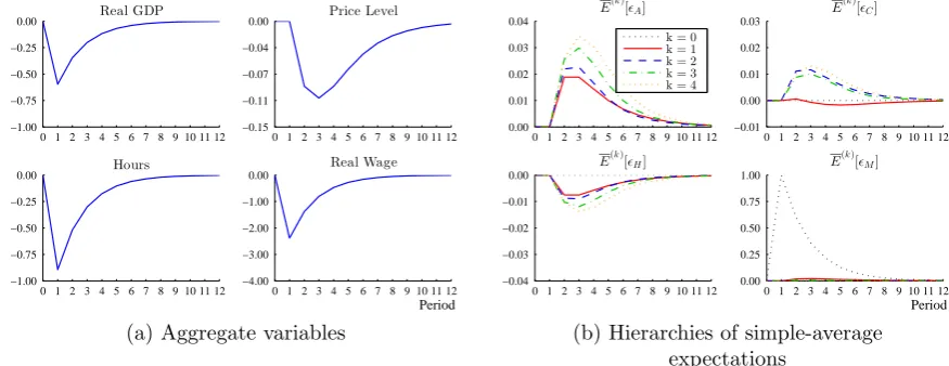
2.1 The hierarchy of simple-average expectations (x(0:_t_|_tk∗)) following a one standard deviation shock to the underlying state with no network (q = 0) 54 2.2 The hierarchy of simple-average expectations (x(0:_t_|_tk∗)) following a one standard deviation shock to the underlying state with agents each ob-serving one competitor (q= 1). . . 55

2.3 Varying the number of other agents observed (q). . . 56

2.4 Varying underlying persistence (ρ) . . . 57

2.5 Varying the relative innovation variance (σ_v2/σ2_u) . . . 57

2.6 The hierarchy of simple-average expectations (x(0:_t_|_tk∗)) following a one standard deviation network shock (a one standard deviation shock to e vt and the corresponding conditional expected value for higher-weighted averages) with agents each observing one competitor (q= 1). . . 58

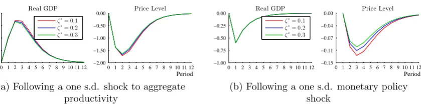
2.7 Varying the degree of network irregularity (ζ∗) . . . 59

2.8 Varying the relative innovation variance (σ2 v/σ2u) . . . 60

2.9 Varying underlying persistence (ρ) . . . 61

3.1 IRFs following a one s.d. shock to firms’ aggregate productivity . . . 122

3.2 IRFs following a one s.d. shock to the utility of consumption . . . 123

3.3 IRFs following a one s.d. shock to the disutility of labour . . . 124

3.4 IRFs following a one s.d. monetary policy shock . . . 124

3.5 IRFs for various numbers of competitors observed . . . 124

3.6 IRFs for various degrees of network irregularity . . . 125

3.7 IRFs for different levels of relative signal variance . . . 126

3.8 IRFs following a one s.d. shock to _evA,t . . . 127

3.9 IRFs following a one s.d. shock to _evW,t . . . 128

3.10 IRFs following a one s.d. shock to _evY,t . . . 128

3.11 IRFs for various numbers of competitors observed . . . 129

(10)

List of Figures

3.13 IRFs for different levels of relative signal variance . . . 130

3.14 IRFs for aggregate shocks with indicative bands for network shocks . . . 131

4.1 The Lambert _W and Wright ω functions in the real domain. Both plots include the 45◦ line for reference. . . 172

4.2 Optimal price under full-information by nominal marginal cost. . . 174

4.3 Optimal price under full-information by a weighted average of other firms’

prices. . . 175

4.4 Optimal price under full-information by base market share. . . 176

4.5 IRFs for the three systems of demand . . . 188

4.6 Hierarchies of simple-average expectations following a TFP shock . . . . 190

4.7 Hierarchies of simple-average expectations following a monetary policy shock. . . 191

4.8 Responses to a 1 s.d. shock to vfA

t . . . 193

(11)

List of Tables

2.1 Size (each) of F, U, V and W, assuming use of double-precision. . . 48

2.2 Baseline parameterisation . . . 54

3.2 Share of unconditional variance attributable to network shocks (%) . . . 132

(12)

Chapter

1

Introduction and common definitions

1.1

Introduction

This thesis is interested in two fundamental questions of macroeconomics. First, what are the underlying causes of observed volatility in aggregate variables? From where do the shocks arise and of what are they comprised? Second, what explains the magnitude and persistence of the effects of aggregate shocks on the macroeconomy? Is it possible for those effects to persist beyond the shock itself, or beyond the time when agents in the economy successfully identify it?

These are by no means new questions – macroeconomists have been grappling with them for decades – but they remain open questions of active research and recent work has brought each of them (and previous attempts at answering them) into a new light.

(13)

1.1. Introduction

large. Section1.3below offers a formal definition of such a distribution, demonstrates why it allows for idiosyncratic shocks to have aggregate effects and discusses the class of distributions that meet such a characteristic.

The second question is of particular importance to a policy maker seeking to dampen aggregate volatility in an economy. Statistical analyses, relying only minim-ally, if at all, on economic theory, have suggested that the effects on real GDP and aggregate prices from identified aggregate shocks, both real and nominal, are signi-ficant and quite persistent. Understanding why this is so, particularly for nominal shocks, is therefore of critical importance.

The most obvious way to model rigidity in aggregate prices is naturally to suppose that individual prices are themselves in some way “sticky.” This approach was supported by early quantitative evidence, which suggested that prices, once set, generally remained fixed for 12 months (Taylor, 1999). With this in mind, the canonical New Keynesian model was developed by assuming that firms follow simple

time-based pricing rules. That is, that firms choose only the magnitude of any price

changes, while the timing of those changes is determined exogenously. Standard approaches here are the staggered pricing rule of Taylor (1980), in which firms’ prices remain fixed forn periods and a fraction 1/n of firms update their prices each period, and the model ofCalvo (1983), in which a random fraction of firms are able to update in each period. Since simple models of state-based pricing, such as those proposed by Rotemberg (1982), imply similar Phillips curves under linearisation, it was generally held that the analytically simple time-based rules were sufficient.

However, a variety of challenges to simple time-based pricing rules have arisen in recent years. From a theoretical perspective, models that exogenously impose the timing of price changes would appear to fail the Lucas Critique by assuming, rather than deriving, policy invariance in agents’ actions (e.g. Plosser, 2012). In-deed, modern models of state-based pricing (i.e. that look both at the magnitude of price changes and whether and when to change) have consistently shown that

selec-tion effects work against any persistence of aggregate effects on real variables, with

(14)

1.1. Introduction

Empirically, a variety of modern studies of microeconomic price changes have demonstrated that a great many prices are remarkably short lived. The seminal work of Bils and Klenow (2004), for example, found that the median duration of prices in CPI data in the United States was 4.3 months, an update frequency almost three times higher than previously thought. More recent work by Klenow and Kryvtsov

(2008) found a median duration of only 3.7 months and highlighted that a significant fraction of goods’ prices are changed on a weekly basis.

With prices apparently quite flexible and selection effects ensuring minimal real effects via what individual price stickiness remains, it is therefore conceptually ne-cessary to develop models of real rigidity – a “contract multiplier,” in the words of

Taylor(1980) – to explain the sluggish responses observed in aggregate price indicies following monetary shocks.

One key approach to achieving real rigidities in firms’ pricing is to suppose that they have imperfect access to information, an idea that dates to Lucas (1972) and

Phelps (1984). Modern models in this field fall broadly into three categories:

1. Sticky Information. First, as argued byMankiw and Reis (2002), firms may have access to information only infrequently, so that in aggregate, they only respond to a policy change gradually. Reis (2006) provides a microfoundation for this idea, arguing that information processing costs (as distinct from classic menu costs) make it optimal for firms to delay their updates.

2. Rational Inattention. Second, as suggested by Sims (2003), firms may be subject to an information processing constraint, whereby there is a limit to the amount of information they can accommodate, irrespective of the cost of doing so. In such a case, it is rational for firms to access information in every period, but to select which signals to observe.

(15)

1.1. Introduction

Common Knowledge,” with firms needing to consider the higher-order beliefs of their competitors.

The work of this thesis fits squarely in the latter of these categories, extending the problem to scenarios where firms must consider not just the simple average of other firms’ expectations, but weighted averages as well. The sizes of firms’ state vectors become much larger in these settings and their signal extraction problems become correspondingly more difficult, thus leading to more sluggish responses in prices following aggregate shocks, even when firms are free to update their information sets and their prices every period.

(16)

1.2. Higher-order expectations

1.2

Higher-order expectations

The near-ubiquitous treatment of higher-order expectations in the macroeconomic literature to date1 _{has been to consider only the hierarchy of} _{simple average}

ex-pectations. That is, to consider settings in which agents are interested only in the sequence of objects xt, Et[xt], Et

Et[xt]

,_{· · ·} where Et[·]≡ R1

0 Et(i) [·]di.

It is important to realise that this is a modelling choice only, made for analytical convenience. It is easy to envisage scenarios where other, more complex hierarchies of beliefs are relevant and this thesis occupies itself with two such examples. The first, dealt with in chapters 2 and 3, involves rational learning over a network, in which economic agents must (in principle, at least) form opinions regarding the beliefs of every other agent in the network and know that they will each, in turn, do the same. The second, addressed in chapter 4, examines firms’ price-setting problem when household preferences are non-uniform, so that every firm must consider two separate aggregations of belief, one of which is firm-specific.

To model these fully, we therefore first provide a generalised definition of a hier-archy of expectations.

Definition 1. A compound expectation is a weighted sum of all agents’

expect-ations. Let xt be an (m×1) vector of random variables, E[xt|It(i)] be the

ex-pectation of xt conditioned on the period t information set of agent i and Et[xt] ≡

h

E[xt|It(1)] · · · E[xt|It(N)] i

be the (m_×N) matrix containing all agents’

ex-pectations of the same. Let w be an(N _×1) vector of weights across all agents such

that wi ∈[0,1] and

PN

i=1wi = 1. The compound expectation, Ew,t[xt], is given by:

Ew,t[xt]≡ Et[xt]w (1.1)

Note that this nests both simple, or unweighted, average expectations (e.g. wA= h

1

N · · ·

1

N i0

) and individual expectations (e.g. wB = h

00 1 00

i0

).

Definition 2. Let W _≡hwA wB · · · i

be the (N _×p) matrix formed of all weights

of interest in a given problem and p be the number of those weights (i.e. the number

1_{Modern macroeconomic literature on higher-order expectations dates to} _Townsend ₍₁₉₈₃_),

(17)

of columns in W). We then define higher-order expectations as follows, using a

blackboard-bold_E(k) to denote the vector containing all expectations of thek-th order:

E(0)t [xt]≡xt

E(tk)[xt]≡ 

   

EwA,t h

E(tk−1)[xt] i

EwB,t h

E(tk−1)[xt] i .. .     

=vec_Et h

E(tk−1)[xt] i

W _∀k_≥1 (1.2)

Note that if we are interested in pdifferent compound expectations, there are pk

different permutations of k-th order expectations. For example, if xt is scalar and

p= 2, then the vector describing the set of second-order expectations will be of size (4_×1) and arranged in the following way:

E(2)t [xt] = 



EwA,t h

E(1)t [xt] i

EwB,t h

E(1)t [xt] i  =      

EwA,t "

EwA,t[xt]

EwB,t[xt] #

EwB,t "

EwA,t[xt]

EwB,t[xt] #      

Definition 3. A hierarchy of expectations, from order 0to k, is defined recurs-ively as:

E(0:t k)[xt] =        xt

EwA,t h

E(0:t k−1)[xt] i

EwB,t h

E(0:t k−1)[xt] i .. .        (1.3)

Note that this is not simply the stacking of each order of expectations on top of each other. For example, if xt is scalar and p= 2, the hierarchies (0 : 1) and (0 : 2)

(18)

E(0:1)t [xt] = 

 

xt

EwA,t[xt]

EwB,t[xt] 



 E

(0:2)

t [xt] =              xt

EwA,t 

 

xt

EwA,t[xt]

EwB,t[xt] 

 

EwB,t 

 

xt

EwA,t[xt]

EwB,t[xt]                

The benefit of depicting hierarchies in this recursive manner is that it becomes simple to extract sub-hierarchies comprised of a single compound expectation. For example, ifwA =

h

1

N · · ·

1

N i0

so thatEwA,t[xt] =Et[xt] is the average expectation, the

sub-hierarchy ofx(0:_t k) _≡x_t0, Et[x0t], Et

Et[x0t]

,_{· · ·}0 may be extracted as:

x(0:_t k) =hI 0

i

E(0:t k)[xt]

In all of the models in this thesis, the expectation hierarchy_E(0:_t ∞)[xt] will represent

the unknown state vector about which agents attempt to learn.

1.2.1

Size of the expectation hierarchy

Although not of particular importance in theory, the size of the state vector of in-terest is of crucial importance if any model is to be simulated. It is clear that if xt

containsmelements, then_E(_tk)[xt] – the set ofk-th order expectations – will contain

mpk _{distinct elements. However, it is worth emphasising that it does not in}

gen-eral follow that the hierarchy_E(0:_t k∗)[xt] will contain m

Pk∗ k=0pk

unique elements. This is because if one of the compound expectations, say EwB [·], is formed from a

single information set – i.e. a single agent’s expectation – then the law of iterated expectations implies that EwB,t[EwB,t[xt]] =EwB,t[xt].

(19)

number of unique elements in the hierarchy _E(0:_t k∗)[xt] will be given by:2

N(m, p, q, k∗) = m pk∗+

k∗₋₁ X

k=0

pk₋q

k X

s=0

ps

!!

(1.4)

with N(m, p,0, k∗) = mPk∗ k=0p

k_{. Nevertheless, even when} _q ₌ _p_{, it should be}

readily apparent that size of an expectation hierarchy explodes in bothp(the number of compound expectations) and k∗ (the highest order in expectations). Figure 1.1

illustrates this point, plotting the size of the hierarchy whenq = 0 andm = 1.

A state vector of infinite dimension need not be a problem, per se, provided that the researcher is able to make a reasonable approximation of agents’ actions by restricting attention to a finite subset of the state. In most models – including those of this thesis – imposing a finite upper limit, k∗, on the number of orders of expectation will be acceptable as in order to ensure stability in agent actions, decreasing weight is placed on higher order expectations.

On the other hand, allowing the number of relevant compound expectations to increase can be more problematic as there is rarely, if ever, an obvious reason for weighting them differently. Existing work in the macroeconomic literature has gen-erally avoided this difficulty by limiting attention to problems that implicitly assume that p= 1 (in particular, that all agents care only about the simple average expect-ation of their competitors).

This avenue is not available when considering learning via networks, however, where it is typically the case thatp is given by the number of agents in the network, or in the case of asymmetric preferences examined in the final chapter, where p is given by the number of firms in the joint demand system.

2

m



 [1] |{z}

0-th order

+ [p] |{z}

1-st order

+

p2−q | {z }

2-nd order

+

p∗ p2−q

−q

| {z }

3-rd order

+

p∗ p∗ p2−q

−q

| {z }

4-th order

+· · ·





=m

k∗

X

k=0

pk

!

−q

k∗

−1

X

k=0

k

X

s=0

ps

!!

(20)

0

2 4

2 0

p

6 10

8 6 4

k*

8 0 10 500

N

1000

(a) Linear scale

0

2 4

4 8

8 0 10

10 6

p

6

k*

2 0

10

ln(N)

20

(b) Log scale

1 2 3 4 5 6 7 8 9 10

1 10 100 1000 10000

k*

p = 1

p = 2

p = 3 p = 4

p = 5

(c) Cross-section byp(log scale)

1 2 3 4 5 6 7 8 9 10

1 10 100 1000 10000

p

k* = 1

k* = 2

k* = 3 k* = 4

k* = 5

[image:20.595.114.546.253.579.2]

(d) Cross-section by k∗ _{(log scale)}

(21)

1.3. Asymptotically non-uniform distributions

1.3

Asymptotically non-uniform distributions

The second key theme of this thesis is an illustration of how idiosyncratic shocks need not “wash out” and may, instead, induce aggregate volatility in an economic context. Fundamentally, this implies an exploration of settings in which the standard law of large numbers does not apply which, in turn, implies that the models must considerweighted sums of agents’ idiosyncratic shocks.

Identifying laws of large numbers for weighted sums of i.i.d. random variables (i.e. the limiting behaviour ofPN

i=1aN,iXi whenE[X] = 0) remains an area of active

research.3 _{However, we do not require an exact characterisation of the necessary}

conditions for a weighted sum to converge to zero, as there is a broad range of functions for the weights under which a weighted sum will not converge to zero. In particular, it is sufficient to suppose that the weights are asymptotically non-uniform:

Definition 4. Let ΦN be a discrete distribution with corresponding p.d.f.4 φN(i).

Let ζ(N) _≡ PN

i=1φN(i)

2

be the Herfindahl-Hirschman index for the same. The

distribution ΦN is asymptotically non-uniform if:

• limN→∞φN(i) = 0∀i; and

• limN→∞ζ(N) = ζ∗ where ζ∗ ∈(0,1).

To appreciate how such a distribution is sufficient to ensure that idiosyncratic shocks do not wash out, suppose that each agent receives an independent, mean zero shock drawn from a common Gaussian distribution (i.e. one fully characterised by its first and second moments):

v(i)_∼N(0,Σvv) ∀i

3_{See, for example,} _Wu₍₁₉₉₉_),_Sung₍₂₀₀₁_{) or}_Cai₍₂₀₀₆_).

4_{Strictly, for a discrete distribution, it is a probability}_mass_{function. But since we will concern}

(22)

and consider the setting where it is not the simple average of agents’ shocks that matters, but a weighted average:

e

vN ≡ N X

i=1

v(i)φN(i) whereφN(i)∈(0,1) and N X

i=1

φN(i) = 1

Sincev_eN is a linear combination of mean-zero Gaussian variables, it must itself have

a Normal distribution with a mean of zero. Its variance will then be given by:

V ar[v_eN] =V ar " _N

X

i=1

v(i)φN(i)di #

=

N X

i=1

V ar[v(i)φN (i)]di

=

N X

i=1

ΣvvφN(i)2di

=ζ(N) Σvv

where in moving to the second line we use the independence of each vector to ignore the covariance terms. The limiting variance asN _{→ ∞}is thereforeζ∗Σvvand, hence,

so long as ζ∗ ₆= 0, the law of large numbers does not apply.

The set of asymptotically non-uniform distributions is quite broad, but in par-ticular it includes the discrete power law distribution (the Zipf distribution)

φN(i) =cNi−γ; wherecN = N X

i=1

i−γ

!−1

and γ >1

and its equivalent for infinite N, the Zeta distribution. The shape parameter,γ >1, governs the scaling of the distribution’s tail, with larger values of γ corresponding to greater non-uniformity. Figure 1.2 plots the values of ζ∗ for a range of values of γ for the Zeta distribution.5

This thesis explores two separate settings in which power law distributions are of economic importance. The first, studied in chapters 2 and 3 relates to social

(23)

1 2 3 4 5 6 7 8 9 10 0

0.1 0.2 0.3 0.4 0.5 0.6 0.7 0.8 0.9 1

[image:23.595.238.403.126.266.2]

γ ζ∗

Figure 1.2: A plot of ζ∗ for power law distributions with shape parameterγ

networks. A great many observed networks, from links between pages on

Wikipe-dia to established relationships in social networks, have been shown to have degree distributions6 _{well approximated by power law distributions (i.e. the networks are}

scale free). See, for example, the work of Albert and Barab´asi (2002), Jackson and

Rogers (2007) orClauset, Shalizi, and Newman (2009). The second setting, studied in chapter 4, relates to the distribution of firm sizes, which has also been shown to follow a power law. See Axtell (2001) or Gabaix (2011).

It is important to appreciate, though, that the models in this thesis do not gen-erally assume any particular distribution, only that it remains non-uniform (in the sense of definition 4) as the support of that distribution grows arbitrarily large.

6_{In network theory, the}_degree _{of a node is the number of connections it has to other nodes, so}

(24)

Chapter

2

Social learning over an opaque

network

Abstract

I present a flexible and readily implemented linear model of rational (i.e. Bayesian) social learning over a network where agents do not know the full structure of the network, but do know the link distribution. I assume that there are several dynamic state variables to be estimated; agents act repeatedly and simultaneously; and agents’ payoffs depend both on the accuracy of their beliefs regarding the state and the proximity of their actions to those of their competitors (i.e. there is strategic interaction). When the network is suffi-ciently irregular, transitory idiosyncratic shocks will not wash out in aggrega-tion but will instead have persistent aggregate effects, and an AR(1) process for the underlying state will induce an ARMA(1,1) law of motion for the hierarchy of aggregate expectations.

2.1

Introduction

2.1.1

Context

An ideal model of network learning must contain a number of key features. Naturally, there must exist a hidden state of the world and agents be arranged in some sort

of observation network, whereby they are informed of the actions, if not the actual

beliefs, of a subset of their compatriots. Beyond this, there are arguably three desirable attributes of a “true” model of network learning:

(25)

2.1. Introduction

2. agents update their beliefs in a Bayesian (i.e. rational) manner; and

3. agents act strategically, with their payoffs a function of other players’ actions.

The complexities involved in solving such a model, let alone simulating it or nesting it within a broader model of the economy, have typically been thought to be sufficiently great as to preclude comprehensive analysis in anything other than trivially small networks. As such, the literature to date has proceeded by avoiding one or more of the above assumptions.1

Early work in observational learning, for example, focussed onsequential learning, with each agent making a single, irrevocable decision in an exogenously defined order, typically after observing the actions of all, or a well-defined subset, of their predecessors. In such a setting, it is well known that agents can rationally (in the Bayesian sense) exhibit “herding”, or “information cascades”, whereby their private signals regarding the unknown state are swamped by the weight of past actions (see, for example,Banerjee, 1992;Lee, 1993; and Smith and Sørensen, 2000).

More recently, work in sequential learning has examined situations where the observation neighbourhood of each agent is determined stochastically. Banerjee and Fudenberg (2004), for example, demonstrate that convergence will occur if the sampling of earlier players’ beliefs is “unbiased” in the sense that it is representative of the population as a whole and at least two earlier players are sampled. More gen-erally, Acemoglu, Dahleh, Lobel, and Ozdaglar (2011) characterise the (Bayesian) equilibrium of a sequential learning model for a general stochastic sampling pro-cess. They demonstrate that so long as no group of agents is excessively influential, there will be asymptotic learning of the truth when private beliefs are unbounded2 and characterise some settings under which asymptotic learning still emerges when private beliefs are bounded.

Although this more recent work carries the flavour of network learning in that agents observe the actions of only a subset of their competitors,3 they do not meet the

1_{Acemoglu and Ozdaglar} ₍₂₀₁₁_{) provide a recent review.}

2_{That is, where agents may receive arbitrarily strong signals so that the support of their}

pos-terior belief that the state is equal to a given possibility is [0,1].

3_Indeed,_{Acemoglu, Dahleh, Lobel, and Ozdaglar}₍₂₀₁₁_{) refer to their model as one of learning}

(26)

2.1. Introduction

popular conception of network learning in which agents undertake repeated, simul-taneous actions in an environment of strategic interaction. Tackling such a problem, however, is notoriously difficult. The presence of strategic interaction introduces the need to consider the infinite hierarchy of higher-order (average) beliefs. When agents exist in an observation network, it is also necessary for each of them to consider the specific belief held by their observation target and, in turn, the belief of their target’s target and so forth. As the number of agents in the network expands, this causes an explosion in the size of the state vector quite apart from the presence of higher-order expectations (see section 1.2 in the previous chapter for more detail), thereby subjecting the problem to the famous curse of dimensionality.

In order to analyse learning in a repeated, simultaneous action environment, the literature has therefore most commonly chosen to abandon the assumption of Bayesian updating. Non-Bayesian learning over a network is typically modelled in the style ofDeGroot(1974), with agents applying a constant weight to their observa-tions of competitors’ acobserva-tions. For example, DeMarzo, Vayanos, and Zwiebel (2003) explore situations where agents assume that signals they receive from observing each other containentirely new information. In a setting where a finite number of agents wish to estimate an unknown, but fixed state θ _∈ _RL_{, they suppose that agents}

each receive a single, conditionally independent and unbiased signal of the state and then communicate their beliefs over multiple rounds. Imposing the assumption that agents update their beliefs via a simple and constant weighted sum greatly simplifies analysis, but introduces what the authors label “persuasion bias” from the agents’ failure to properly discount the repetition of information they receive.

Calv´o-Armengol and de Mart´ı(2007) extend this setting to provide an assessment of the welfare losses from “unbalanced,” or irregular4 networks.

Golub and Jackson (2010) likewise study learning in a setting where agents “na¨ıvely” update their beliefs regarding a fixed state of the world by taking weighted averages of their neighbour’s opinions. In contrast to earlier work, they are able demonstrate that with such heuristic learning, individual beliefs converge to the truth for a broad variety of networks (provided they are sufficiently large) and provide

4_{A regular network is one in which all nodes have the same number of inbound and outbound}

(27)

2.1. Introduction

upper and lower bounds on the rate of convergence.

In the area of what might be called “true” Bayesian network learning (repeated simultaneous actions with agents engaged in Bayesian updating), there has been remarkably little work to date. Gale and Kariv (2003) examine Bayesian network learning in a setting with connected networks5 and in which agents’ payoffs depend only on the proximity of their expectation to the state (i.e. without any strategic interaction). They note that the “computational difficulty of solving the model is massive even in the case of three persons.” Mueller-Frank (2013) details a formal structure for Bayesian learning over an undirected social network (i.e. with pairwise sharing), allowing for a choice correspondence from information to actions (and gen-eral strategies for the selection between indifferent options) as opposed to outright decision rules, but notes the extreme practical difficulties of actually implementing such a rule, both for the agents in principle and the researcher more generally.

Furthermore, both Gale and Kariv (2003) and Mueller-Frank (2013) step away from consideration of strategic interaction in agents’ decision-making, so that when observing any competitor, every agent knows that their action is driven entirely by their belief regarding the underlying state.

2.1.2

This paper

In contrast to earlier work, the present paper is able to embrace all three of the assumptions listed above by combining them with a fourth: network opacity. By denying agents knowledge of the exact topology of the network (the network is

opaque) and instead supposing that they know only the (i.i.d.) distribution from

which observation targets are drawn and do not learn about the structure of the network over time, agents’ state vector of interest includes an infinite sequence of

weighted average expectations instead of individual agents’ expectations. Because

of the recursive nature of agents’ learning, this sequence will be of decreasing im-portance to the hierarchy of simple-average expectations, so an arbitrarily accurate approximation of the full solution may then be found by selecting a sufficiently high

5_{In this context, a connected network is one in which information is able to flow}_from_{any agent}

(28)

2.1. Introduction

cut-off for the number of weighted-average expectations to include, together with the standard cut-off for the number of higher-orders of expectation.

The imposition of an opaque network is both intuitive and appealing. It is not plausible, for example, to suppose that every business knows to whom every other

business speaks, just as nobody knows the identity of all of their friends’ friends. From the researcher’s perspective, this ignorance of topology makes it particularly challenging when attempting to consider the aggregate effects of network learning. But by recognising that not only the researcher but also the economic agents them-selves are ignorant of the network structure, we are able to identify laws of motion for the agents’ aggregate beliefs, even if we can never pin down the path of any individual’s expectation.

The second requirement mentioned above – that agents not learn about the struc-ture of the network over time – may be thought of in two ways. First, one might consider a setting in which the network is dynamic, changing every period. In

ex-tremis, this would involve the network being destroyed and redrawn each period and

in such a scenario, agents are not able to learn about the network as it does not persist over time. The decisions followed by agents will then be fully rational in that they are entirely model-consistent, but the extent to which it might realistically be considered a “network” is called into question.6 Second, one might suppose that the network was drawn once, at time zero, but agents are boundedly rational in that they do not attempt to learn about it beyond the common knowledge of the distribution from which it was drawn. In this setting, agents’ decisions are perhaps best described as conditionally rational, in that conditional on the structure of the network, they are rational in their processing of the information they gain from it.

With unobserved aggregate variables following an AR(1) process, we demonstrate that the full hierarchy of agents’ aggregate expectations will follow an ARMA(1,1) process, with current and lagged weighted sums of agents’ idiosyncratic shocks en-tering at an aggregate level. For sufficiently irregular networks – i.e. where some agents’ actions are disproportionately observable – these weighted sums are shown to

6_{Such a setup, which is indeed deployed in this chapter, might arguably be better thought of}

(29)

2.1. Introduction

not converge to zero, thereby adding aggregate volatility to the system. Despite idio-syncratic shocks being purely transitory, the aggregate volatility they induce through the network is also shown to exhibit (endogenous) persistence.

Because we examine a setting with a dynamic underlying state and demonstrate a specific law of motion for the hierarchy of average expectations, the researcher is able to simulate the aggregate effects of network learning7 without a need to simulate individual agents’ decisions. This makes the model particularly amenable to nesting within broad general equilibrium models of the economy.

Methodologically, this chapter expands on the work of Nimark (2008, 2011a,b), who in turn extended that ofWoodford(2003). The latter of these reintroduced the ideas ofLucas(1972) and Phelps(1984) – that imperfect information could give rise to nominal shocks having real effects – and demonstrated that with incomplete in-formation and strategic interaction, firms become interested in higher-order beliefs. In particular, with firms observing independent, unbiased signals of nominal GDP, Woodford demonstrated aggregate rigidity broadly equivalent to that produced by

Calvo (1983) pricing. In contrast, Nimark (2008) supposed that firms’ uncertainty surrounded the supply side of the economy (the average marginal cost) and, in addi-tion to their private signals, granted firms visibility of the previous period’s aggreg-ate price level. Because aggregaggreg-ate variables are functions of the entire hierarchy of average expectations, this addition required the development of a new solution meth-odology that the present chapter adapts and extends to the idea of agents observing the previous-period actions of specific competitors.

Although the present chapter borrows from these papers and the next chapter applies the current model to a setting of firms’ price-setting behaviour, the model developed here is context free and may be applied to any general setting with strategic competition and network learning. The conclusion considers a number of examples of such applications.

The remainder of this chapter is organised as follows. Section 2.2 presents the model, together with a characterisation of the solution and a methodology for finding

7_{The model is calibrated by two additional parameters: one specifying the number of other}

(30)

2.1. Introduction

(31)

2.2. The Model

2.2

The Model

We here develop a generalised model of Bayesian learning across opaque, stochastic networks with agents’ optimal decision rule depending on both their expectation of the underlying state and their expectation of the agents’ average action. The underlying state is assumed to be subject to persistent AR(1) shocks, while agents’ observations include errors that are entirely transitory Gaussian white noise. It is demonstrated that for an irregular observation network, the hierarchy of aggregated expectations regarding the underlying state follows an ARMA(1,1) process, with weighted sums of agents’ idiosyncratic shocks entering at the aggregate level (i.e. idiosyncratic shocks do not wash out).

A simple roadmap of how this section will proceed may be of some assistance. First, in subsection2.2.1, we will describe the agents’ problem, the information avail-able to them and how they make their decisions. Subsection 2.2.3 will characterise agents’ average action and briefly describe the informational assumptions used in previous research and how they differ to the current paper. Subsection 2.2.4 then explores the process of observing the actions of individual competitors before sub-section2.2.5 presents the main result of this paper.

2.2.1

The general setting

There is a countably infinite number of agents,8 _{indexed in a continuum between}

zero and unity.9 _The _{underlying state} _{follows a vector autoregressive process:}

xt=Axt−1+Put (2.1)

where ut is a vector of shocks with mean zero, while A and P are appropriately

dimensioned matrices of fixed and publicly known parameters. Agents do not observe the value of xt and must instead form beliefs about it. We define Xt to be the

hierarchy of expectations regarding xt, in the sense of definition 3, and refer to it as

8_{An infinite number of agents is assumed to allow an appeal to relevant laws of large numbers}

when considering simple averages of zero-mean shocks.

9_{The assumption of indexing agents from zero to one is innocuous and made only to simplify}

the calculation of averages (e.g. gt=

R1

(32)

2.2. The Model

the state vector of interest.

Xt ≡E

(0:∞)

t [xt] (2.2)

At a minimum,Xt containsxt and the hierarchy of at least one compound

expecta-tion. For illustrative purposes, we will assume that agents’ primary concern is with the the hierarchy of simple-average expectations, so that

x(0:_t_|_t∞) _∈Xt where x

(0:∞)

t|t ≡

h

x0_t Et[xt]

0 Et

Et[xt] 0

· · ·i

0

but it will be shown below that Xt must include a variety of other compound

ex-pectations as well.

Agents’ decision rule

Agents determine their individual actions simultaneously and according to a common linear decision rule:10

gt(i) = λ01Et(i) [Xt] +λ02xt+λ03vt(i) (2.3)

whereEt(i) [·]≡E[·|It(i)] is agenti’s (first-order) expectation of the element within

the square brackets conditional on all information available to her in periodt(defined below); and vt(i) is a transitory, mean zero shock specific to agent i in period t

(defined below).

Non-zero elements in λ1 against higher-order average expectations capture

stra-tegic considerations in agents’ actions. Note that the terms in xt and vt(i) are

included here to make the model as general as possible. They allow for the possib-ility that components of i’s signal vector may have direct economic significance in addition to their informational role. Note, too, that althoughxt may be included in

agents’ decision rule, it is not directly observed.11

10_{The derivation of the decision rule will invariably be context-specific. For example, in the}

context of price-setting to be explored in the next chapter, the underlying state will include aggreg-ate shocks to marginal cost and demand, while agents’ actions will be the price they choose and the signal they receive will include their private marginal cost and the previous-period price of a competitor.

11_{For example, a firm may privately observe their productivity, which includes both aggregate}

(33)

2.2. The Model

Equation (2.3) is a reduced form expression for agents’ actions that nests a wide array of commonly studied settings. An illustrative example with a univariate state is considered in depth in section2.3below, while other applications and their implied decision rules are discussed in section 2.4.

Agents’ information

Agents possess common knowledge of joint rationality, in the sense ofNimark(2008), so that they are aware of the structure and the coefficients of the system. Their information sets then evolve as:

I0(i) = {Ω,Φ} It(i) ={It−1(i),st(i)} (2.4)

where Ω is the set of all system coefficients, st(i) is the signal vector received each

period and Φ : [0,1] _→ [0,1] is the (cumulative) distribution from which agents’ observation targets in the network are drawn, assumed to be identical and independ-ent, both across agents and across time. Φ (i) is absolutely continuous over the range [0,1] and has p.d.f. φ(i).

Each agent’s signal vector is made up of two, distinct components – a

pub-lic/private signal based on the underlying state and a social signal derived from

observing competitors’ actions with a one-period lag:

st(i) = "

sp_t(i)

ss t(i)

#

(2.5)

sp_t(i) = D1xt+D2Xt−1+R1vt(i) +R2et+R3zt−1

ss_t(i) = gt−1(δt−1(i))

Public/Private signalsmay include both current and lagged information12_and

are noisy, including three sources of uncertainty:

• vt(i) is a vector of transitory shocks specific to agent i in period t, drawn

from independent and identical Gaussian distributions with mean zero and variance Σvv. These may simply be noise in agents’ private signals or may

carry economic significance, depending on the context.

(34)

2.2. The Model

• ztis a vector ofnetwork shocks(see equation2.12below), comprised of weighted

sums of all agents’ idiosyncratic shocks.

• et is a vector of transitory “noise” shocks to public signals, drawn from an

independent Gaussian distribution with mean zero and variance Σee.

Note that although agents may observe signals based on the current underlying state (xt), they do not observe signals based on the current hierarchy of expectations

about the state (Xt). This is because to do so would involve agents observing a signal

based on their beliefs before they have even formed them! However, we include terms in Xt−1 and zt−1 (instead of just xt−1) to allow agents to observe, with a lag,

aggregate variables and thus the past effect(s) of their network learning.

Social signals are observations of the previous-period actions of specific agents, with the function δt mapping each agent onto their observation targets:

δt: [0,1]→[0,1] q

(2.6)

whereq is the number of agents observed. In other words, δt(i) is the result of i’sq

separate draws from Φ for period t. For presentational simplicity, we will typically assume that q = 1 (i.e. that all agents observe a single other agent) and simply write j = δt(i) to mean that agent j’s period-t action will be observed by agent i

(in period t+ 1). To speak of the observee of an observee, we write δs(δt(i)): the

identity of the agent whose period-s action is observed by the agent whose period-t action is observed by agent i.

With agent i observing the previous-period action of a single competitor, their social signal is therefore given by

ss_t(i) =gt−1(δt−1(i))

=λ0₁Et−1(δt−1(i)) [Xt−1] +λ02xt−1+λ03vt−1(δt−1(i)) (2.7)

2.2.2

The observation network

Because agent i’s social signal is based on her observee’s expectation, Bayesian up-dating then requires thati includeEt(δt(i)) [Xt] in her own state vector of interest.

(35)

2.2. The Model

ialso maintain an estimate of Et(δt(δt(i))) [Xt], and so forth. This is the explosion

of the state vector inp (the number of compound expectations) described in section

1.2 of the previous chapter. In order to make the problem tractable, we make two key assumptions:

Assumption 1. The network is stochastic and opaque, in that:

• all agents observe the same number of other agents;

• observees are drawn from identical, fully independent distributions with p.d.f.

φ(i);

• agents know the identities of the other agents they observe;

• agents do not know who they are observed by; and

• agents do not learn about the network topology over time.

To obtain this last point, we suppose that agents make a fresh draw of whom to observe every period, in which case nothing could be learned about the network topology (since it changes every period).

Assumption 2. The network is asymptotically irregular, in that its degree

distribu-tion is asymptotically non-uniform (see definidistribu-tion 4).

As shown in the previous chapter and expanded on below, assumption 2 is suf-ficient to ensure that idiosyncratic shocks do not “wash out” in aggregation and will, in this context, enter into agents’ aggregate beliefs. Social networks are widely regarded as having degree distributions well approximated by power law distribu-tions,13 _{which satisfy this assumption. It is important to appreciate, though, that}

the model here does not require any particular distribution of links in the agents’ network, only that the network remain irregular as it grows arbitrarily large.

13_See_{Albert and Barab´asi}₍₂₀₀₂_),_{Jackson and Rogers}₍₂₀₀₇_{) or}_{Clauset, Shalizi, and Newman}

(36)

2.2. The Model

2.2.3

Agents’ learning and imperfect common knowledge

It will be shown below that the hierarchy of agents’ expectations obeys the following ARMA(1,1) law of motion:

Xt ≡E(0:t ∞)[xt] =F Xt−1+G1ut+G2zt+G3et+G4zt−1 (2.8)

wherezt is a vector of transitorynetwork shocks, derived as weighted sums of agents’

idiosyncratic shocks. The exact statistical properties of zt are derived below in

proposition 2.

In the macroeconomic literature, this environment – a state space system paired with strategic complementarity – is typically referred to as a setting of incomplete

common knowledge, a phrase coined by Woodford(2003) in his demonstration of the

potential importance of incomplete information in explaining inflation dynamics.

The system described here is not in the form of a classic state space problem, however, both because of the presence of the lagged state in agents’ signals (2.5) and because of the moving average component of the law of motion (2.8). The usual response to these quirks would be to stack the state vector with both its own lag and the lag of the shock with the moving average component, thus creating a combined state that follows an AR(1) process:



 

Xt

zt

Xt−1





=



 

F G4 0

0 0 0

I 0 0



 



 

Xt−1

zt−1

Xt−2





+



 

G1 G2 G3

0 I 0 0 0 0



 



 

ut

zt

et 

 

and then to express agents’ signals in terms of this combined state and estimate the system as a classic filtering problem. This approach more than doubles the size of the state vector, though, which may present problems when simulating the system with finite computing resources (and particularly so in the present setting with multiple compound expectations).

Fortunately, the following lemma grants us that it is not necessary here to include

zt in the state vector of interest.

Lemma 1. Agents’ contemporaneous expectations of the network shocks are zero

(37)

2.2. The Model

Proof. Since all shocks are distributed Normally, the ability of an agent to create an

expectation about a variable depends on the covariance between that variable and the agent’s signal vector. But, by construction, agent i does not observe any signal that is based onzt. Since zt is transitory and fully independent across time and from

the underlying state, it must be the case that Cov(zt,st(i)) =0. The only possible

exception to this is to note that zt is comprised of weighted sums of idiosyncratic

shocks and agent i’s signals do include vt(i). However, we have that:

Cov {1}v_et,vt(i)

=E

"

lim

N→∞

N X

j=1

φN(j)vt(j)vt(i) #

= lim

N→∞φN(i) Σvv

=0

where the second equality relies on the independence of agents’ idiosyncratic shocks and the third on assumption 2 (which grants us that limN→∞φN(i) = 0 ∀i). An

equivalent argument applies to all higher-weighted averages: Cov {q}v_et,vt(j)

.

Since all agents’ expectations of the network shock are zero, it must be the case that all average expectations (simple or weighted) of the network shock are also zero and since agents are jointly rational, this must be common knowledge. There is therefore no need to include any expectation of zt within the state vector to be

estimated.

Because of the linearity of the system, the best linear estimator in the sense of minimising the mean squared error14 will be a Kalman filter:15

Et(i) [Xt] =Et−1(i) [Xt] +K{st(i)−Et−1(i) [st(i)]} (2.10)

whereK is a time-invariant projection matrix (the Kalman gain). As in other models of imperfect common knowledge, sinceXt includesx

(0:∞)

t|t , we have that (a) the state

vector to be estimated is of infinite dimension; and (b) the Kalman filter serves a dual role, both as estimator and as part of the law of motion for the state vector.

14_{With all shocks drawn from Gaussian distributions, it will be the best such estimator, linear}

or otherwise.

15_{A derivation of the standard Kalman filter may be found in most texts on dynamic}

(38)

2.2. The Model

Woodford (2003) supposed that agents (firms) each receive only a private signal regarding the underlying state (aggregate expenditure) and no social signal from other agents. In such a setting, where Xt = x

(0:∞)

t|t , Woodford showed that F will

be lower-triangular: each order of average expectations will be a linear combination of current period shocks and lower order expectations. Consequently, F may be constructed sequentially, first finding an expression for Et(i) [xt], then averaging it

and repeating the process to findEt(i)

Et[xt]

and so forth.

By contrast, Nimark (2008) allowed agents to observe an aggregate signal (the average price) from the previous period in addition to their private signals.16 _This

meant that each agent’s signal vector includes a linear combination of the entire

hierarchy of previous-period expectations (since individual actions are based on

(ex-pectations of) the entire hierarchy). As a result, the solution must be found for all higher-order expectations simultaneously and the state vector of interest expands to includex(0:_t₋∞₁_|_t)₋₁ so thatXt=

h

x_t(0:_|_t∞)0 x_t(0:₋₁∞_|_t)₋0₁i 0

.

An alternative to including x(0:_t₋∞₁_|_t)₋₁ in the state vector of interest is to retain the current signal vector and instead to modify the Kalman filter:

Et(i) h

x(0:_t_|_t∞)i =Kst(i) + (F −K(D1F +D2))Et−1(i)

h

x(0:_t₋∞₁_|_t)₋₁i

This approach was first developed byNimark(2011b) and is also used in the current paper to avoid the need to stack the state vectors of interest.

It is perhaps worth emphasising that the signal structures assumed byWoodford

(2003) andNimark(2008) both result in agents only being concerned with thesimple

average expectation of their peers (or higher-order versions of the same). In the

language of chapter 1, they have chosen signal structures that explicitly set p = 1, thereby having the infinite dimensionality of the state vector arising only from the presence of higher-order expectations.

16_{The hidden aggregate state in}_Woodford₍₂₀₀₃_{) was on the demand side of the economy, while}

(39)

2.2. The Model

2.2.4

Observing individual competitors’ actions

In implementing the Kalman filter (2.10), agentineeds to create a prior expectation of the signal they will receive in the next period. From equation (2.7), we see that it is therefore necessary for agent i to constructEt(i) [gt(δt(i))] as part of her prior

for periodt+ 1, which includesEt(i) [Et(δt(i)) [Xt]]:

Et(i)

ss_t₊₁(i)=Et(i) [gt(δt(i))]

=Et(i) [λ01Et(δt(i)) [Xt] +λ02xt+λ30vt(δt(i))]

ConstructingEt(i) [Et(δt(i)) [Xt]] requires, in turn, that agent itake a view

regard-ing who δt(i) is observing: that is, the action of δt−1(δt(i)).

Proposition 1. Given assumption 1 and common knowledge of rationality, agents’ use of a linear estimator implies that all agents treat all other agents as though they

observe a common, weighted average of previous-period actions, with the weights

given by the distribution φ.

Proof. The proof may be found in appendix2.A.

We see from equation (2.3) that the weighted-average action, _egt, is given by:

e

gt=λ01Ee_t[X_t] +λ0₂x_t+λ0₃ e

vt (2.11)

where Ee_t[·] ≡ R1

0 Et(j) [·]φ(j)dj is the (first-order) weighted-average expectation,

which we will more fully denote {1}

e

Et[·] (see proposition 2 below).

We cannot, in general, make use of some law of large numbers to disregard the effect of idiosyncratic shocks in the weighted-average action – that is, we cannot assume thatv_et≡

R1

0 vt(j)φ(j)dj will be equal to zero – because the weights applied

to each agent may not be sufficiently close to equal. As an extreme example, if all agents were to observe agent 1 and nobody else (i.e. φ(1) = 1 andφ(i) = 0 _∀i₆= 1), we would then have that v_et = vt(1) which in any given period will be non-zero,

almost surely.

(40)

2.2. The Model

Proposition 2. Suppose that vt(i)∼ i.i.d. N(0,Σvv) ∀i, t. For a finite number of

agents (N), define the aggregate statistics

{1}

e

vN,t≡

1 N

N X

i=1

vt(δt(i)) {1}v¨N,t≡ N X

i=1

vt(i)φN(i)

{2}

e

vN,t≡

1 N

N X

i=1

vt(δt(δt(i))) {2}v¨N,t≡ N X

i=1

vt(δt(i))φN(i)

{3}

e

vN,t≡

1 N

N X

i=1

vt(δt(δt(δt(i)))) {3}v¨N,t≡ N X

i=1

vt(δt(δt(i)))φN(i)

..

. ...

Given assumptions 1 and 2, we have the following results in the limit (as N _{→ ∞}):

1. {q}

e

vN,t d

−→{q}

e

vt∀q where vet ∼N

0,Σ{q}

e vev

Σ{q}

e vev

= (1₋(1₋ζ∗)q) Σvv

2. {q}_v_¨

N,t

L2 −→{q}

e

vt∀q

3. Cov {p}v_et,{q}vet

= Σ{p}

e vev ∀

p < q

Proof. The proof may be found in appendix2.B.

Given proposition 2, we refer to {q}v_et as theq-th weighted average of agents’

idiosyncratic shocks and define the vector of network shocks,zt, as that containing

the full sequence of these weighted sums:

zt≡         

{1}

e

vt

{2}

e

vt

{3}

e

vt

{4}

e vt .. .         

∼N(0,Σzz) Σzz =         

Σ{1}

e vev

Σ{1}

e vve

Σ{1}

e vev

Σ{1}

e vev · · ·

Σ{1}

e vev

Σ{2}

e vve

Σ{2}

e vev

Σ{2}

e vev · · ·

Σ{1}

e vev

Σ{2}

e vve

Σ{3}

e vev

Σ{3}

e vev · · ·

Σ{1}

e vev

Σ{2}

e vve

Σ{3}

e vev

Σ{4}

e vev · · ·

.. . ... ... ... . ..          (2.12)

Including these higher weighted averages is necessary because of the recursive nature of agents’ learning through the Kalman filter. It will be shown below that the aggregate expectation{1}

e

Et[Xt] will be a function of{1}vetand

{2}

e

Et−1[Xt−1], the

latter of which will be a function of{2}

e

vt−1 and {3}Ee_t−2[Xt−2], etc.

(41)

2.2. The Model

Corollary 1. Σvv ≥ · · · ≥ Σ

{3}

e vev ≥

Σ{2}

e vev ≥

Σ{1}

e vev

where _≥ is in the sense that the

difference between the two is a positive-definite matrix.

Proof. Trivial, sinceζ∗ _∈(0,1).

Corollary 2. E{q}_evt|{1}evt=a

=a _∀q_≥2

Proof. Follows immediately from item 3 in the proposition.

The first of these is a necessary component of approximating the full solution with a finite state vector (see section 2.2.6 below), while the latter is used when simulating the aggregate effects of network learning.

2.2.5

Social learning over an opaque, irregular network

We are now in a position to present the main result of this chapter.

Theorem 1. Given the broad setting described above and assumptions 1 and 2, the hierarchy of agents’ aggregate expectations will obey the following ARMA(1,1) law of motion:

Xt ≡ 

       

xt

Et[Xt]

{1}

e

Et[Xt]

{2}

e

Et[Xt] .. .



       

=F Xt−1+G1ut+G2zt+G3et+G4zt−1

where

Et[·] =

Z 1

0

Et(i) [·]di

{1}

e

Et[·] =

Z 1

0

Et(δt(i)) [·]di

{2}

e

Et[·] =

Z 1

0

Et(δt(δt(i))) [·]di

(42)

2.2. The Model

Proof. The proof may be found in appendix2.C

Although the complete derivation is provided in the appendix, an outline of the agents’ learning process may be of interest. To begin, we define the matricesSx, Ts

and Twq as the matrices that select xt, Et[Xt] and

{q}

e

Et[Xt] respectively from Xt

(e.g.,Tw2Xt=

{2}

e

Et[Xt]). We also define the general notation thatθt|q(i) represents

the error in agent i’s period-q expectation regarding θt. In particular, we will use

the following:

st|t−1(i)≡st(i)−Et−1(i) [st(i)] : signal innovation

Xt|t−1(i)≡Xt−Et−1(i) [Xt] : prior expectation error

Xt|t(i)≡Xt−Et(i) [Xt] : contemporaneous expectation error

The filter

As with a standard Kalman filter, the Kalman gain (equation 2.30) is calculated as:

Kt=Cov(Xt,st|t−1(i))

V ar st|t−1(i)

−1

where st|t−1(i) is the agent’s signal innovation (the portion of their signal that was

not forecastable). With agents observing the previous-period actions of specific com-petitors, the signal innovation is then able to be expressed (equation 2.36) as:

st|t−1(i) =M1Xt−1|t−1(i) +M2Xt−1|t−1(δt−1(i)) +M3Xt−1

+N1ut+N2vt(i) +N3et+N4vt−1(δt−1(i)) +N5zt−1

Note that innovation in i’s signal includes not only a term in their own previous period expectation error but also a term in theirobservee’s error. As such, both the covariance and variance terms in the Kalman gain will therefore include terms in both the variance ofi’s expectation error, Vt−1|t−1 ≡E

Xt−1|t−1(i)Xt−1|t−1(i)

0

, and the

covariance between any two agents’ errors, Wt−1|t−1 ≡E

Xt−1|t−1(i)Xt−1|t−1(j)

0

.

(43)

2.2. The Model

DefiningM _≡hM1 M2 M3

i

, the full set of equations for updating the filter for one period is given by:

Est|t−1(i)st|t−1(i)

0

=M



 

Vt−1|t−1 Wt−1|t−1 Vt−1|t−1

Wt−1|t−1 Vt−1|t−1 Vt−1|t−1

Vt−1|t−1 Vt−1|t−1 Ut−1





M

0

+ (M1+M2+M3)G2ΣzzN50

+N5ΣzzG02(M1+M2+M3)

0

−M2Kt−1N2ΣvvN40

−N4ΣvvN20K

0

t−1M

0

2

+N1ΣuuN10 +N2ΣvvN20 +N4ΣvvN40 (2.13a)

Est|t−1(i)st|t−1(j)

0

=M



 

Wt−1|t−1 Wt−1|t−1 Vt−1|t−1

Vt−1|t−1 Vt−1|t−1 Ut−1





M

0

+ (M1+M2+M3)G2ΣzzN50

+N5ΣzzG02(M1+M2+M3)

0

+N1ΣuuN10 (2.13b)

EXtst|t−1(i)

0

=F hVt−1|t−1 Vt−1|t−1 Ut−1

i

M0

+G1ΣuuN10

+F G2ΣzzN50

+G4ΣzzG02(M1+M2+M3)

0

+G4ΣzzN50 (2.13c)

EXt|t−1(i)st|t−1(j)

0

=FhVt−1|t−1 Wt−1|t−1 Vt−1|t−1

i

M0

+G1ΣuuN10

+F G2ΣzzN50

+G4ΣzzG02(M1 +M2+M3)

0

(44)

2.2. The Model

Kt=E

Xtst|t−1(i)

0

Est|t−1(i)st|t−1(i)

0−1

(2.13e)

Ut=F Ut−1F0

+G1ΣuuG01+G2ΣzzG02+G4ΣzzG04+F G2ΣzzG40 +G4ΣzzG02F

0

(2.13f)

Vt|t−1 =F Vt−1|t−1F0

+G1ΣuuG01+G2Σz

Incomplete information and the idiosyncratic foundations of aggregate volatility