DEVELOPMENT AND APPLICATION OF A STAGE GATE PROCESS TO REDUCE THE UNERLYING RISKS OF IT SERVICE PROJECTS

ISSN: 1992-8645 www.jatit.org E-ISSN: 1817-3195

ON THE MODELING OF TOURISTS VISIT TO TOURIST

ATTRACTION IN SURABAYA USING NEURAL NETWORK

1

R. PRAWIRO KUSUMO R., 2NUR IRIAWAN

1

Student, Management Information Technology, Department of Management Technology, Institut Teknologi Sepuluh Nopember, Surabaya, Indonesia

2

Prof., Department of Statistic, Faculty of Mathematics and Natural Sciences,

Institut Teknologi Sepuluh Nopember, Surabaya, Indonesia

E-mail: [email protected], 2

[email protected]

ABSTRACT

Tourism has a strategic role in the developing of regional economy and society. Surabaya has some object and tourist attractions potentially attracting foreign and domestic tourists to come to Surabaya. The monthly number of tourist who visits to several tourist attractions in Surabaya shows a pattern as time serially data, seasonal, and could be correlated among them. The traditional vector autoregressive (VAR) would be firstly applied to the data. For the comparison, neural networks (NN) couple with VAR structure as an input is proposed to model this data. This paper shows that this proposed method gives better performance than when the data was directly modeled using VAR only. This research also shows that the increasing number of neurons in the hidden layer does not always give effect to the decreasing the value of MAPE as a tool to differentiate the models.

Keywords: tourism, tourist visit, time series, VAR, neural network

1. INTRODUCTION

Tourism has a strategic role in the development of the economy, especially in increasing foreign exchange earnings, local revenue, providing work opportunities and the chance to improve the public welfare. Based on this information, it appears that the tourism sector is able to boost the pace of economic development of a region through businesses that include in the tourism industries.

Surabaya as a second biggest city in Indonesia, has the tourist attractions that potentially attract foreign tourists and domestic tourists. Surabaya is also known as the city of Heroes since of 10 November 1945 historical event, the time when defending independence against colonialist. In conjunction with that, Surabaya offers several kinds of tourist attractions; including culinary tourisms, historical tourisms, monument tourisms, museum tourisms, religious tourisms, shopping tourisms, nature tourisms, and city park tourisms. The monthly number of tourist who visits to several tourist attractions of Surabaya shows a pattern as time serially data, seasonal and can correlate between tourism attractions. To analyze this kind of data requires special analytical methods, such as vector autoregressive (VAR) and neural network (NN). VAR method is possibly used to describe the

dynamic behavior between the observed variables and each which are interrelated. VAR is frequently suggested as an alternative method to solve the problem when there is more than one serial data which each serial variable has mutual influence on other circumstances.

NN, on the other hand, has been widely applied in many fields that accommodate the computational estimation models. Structure of VAR could be implemented in a NN structure. This is because NN has several advantages: (1) the capability to solve non-linear problems which are common found in the characteristic of the data, (2) the ability to

provide answers for a specific pattern

(generalization), (3) the adeptness to be

automatically learn the numerical data that trained in the network.

ISSN: 1992-8645 www.jatit.org E-ISSN: 1817-3195

connecting among those correlated tourist

attractions.

2. LITERATURE AND METHODOLOGY

2.1 Vector Autoregressive (VAR)

Modelling of multivariate time series by using VAR is one of forecasting method that often used because it is easy and flexible compared to other methods. Applying VAR, the data must be stationary in both mean and variance. In general form, the model VAR(p) can be written as in Equation (1).

⋯ (1)

After estimating the parameters using maximum likelihood (ML), Akaike's information criterion (AIC) method would be employed to select the best model built based on in-sample data. The smaller AIC value, the better the model to represent the data [1]. Mean absolute percentage error (MAPE), on the other hand, will be used to choose the best performance model in forecasting of the future based on out-sample data. Forecasting is usually categorized as very good when the value of MAPE is less than 10% and good enough when the value of MAPE is less than 20% [2]. The formation of the VAR models includes the steps as follows:

1. Model identification. Identification and

checking the stationary data have to be prepared before VAR analysis is employed. It is due to the requirement and assumption of a stationary of VAR. To determine whether the data meets the assumption of a stationary in variance, we can use the Bartlett test. While testing for stationary in mean, the Dickey-Fuller statistics test could be applied [3].

2. Determination Order VAR Model. Model

order determination has to be made to obtain the appropriate VAR model. There could be more than one fitted models. To strengthen the initial presumption, the AIC could be employed to determine the model order. The selected VAR order model that has the smallest AIC value, is considered as the most appropriate model to represent the data.

3. Parameters Estimation and Significance

Test. After identifying the model with the

appropriate order of VAR, the estimating parameters and testing the significance of parameter is the next step. Efficient estimator is estimated by minimizing the square of the difference between the data and its estimated value. Testing the significance of the model parameters must be done to determine the significant parameters in the model. The

elimination of non-significant parameters would lead model to be more parsimony.

4. Testing residuals assumption. There are two

steps of testing. Firstly, test the identical and independent of residual assumption, or white noise test. Residual would fulfil the white noise if it satisfies the two properties, i.e. identical (have a constant variance) and independent (no serially correlated). Secondly, test the multi-normal residual assumption, or multivariate normal distribution test, which can be done by calculating the distance squared of each residual data to the center.

2.2 Neural Network

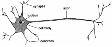
Neural network (NN) represents an information processing system that its characteristics similarly to biological neural networks. A neural network is a distributed parallel processor and has a tendency to store the knowledge acquired from the experience and keeping it available to be used. It resembles the brain in two respects: (1) the knowledge obtained by the network is gathered from a learning process, (2) strength of connections between neurons, known as synaptic weights used to store knowledge [4].

Figure 1: The natural nervous system

An artificial neuron is a computational model inspired in the natural neurons like shown in Figure 1. Synapses that is located on the dendrites or membrane of the neuron, is a natural neuron signals receiver. When the received signals are quite strong (surpass a certain threshold), the neuron will be activated and transmit a signal through the axon. This signal might be delivered to another synapse, and could activate other neurons [5]. When a large number of neurons process signals at the same time, the creatures could solve a complex problem. When there is a new problem that has never been encountered in their life, neurons need to learn from their experiences in the past, then decide the appropriate solution. NN can capture the neurons work that is used to approach a various statistical

models without doing certain hypothesized

relationship between dependent and independent variables. Forms of relationships are determined

ISSN: 1992-8645 www.jatit.org E-ISSN: 1817-3195 accommodate the linear regression model when the

relationship between dependent and independent variables are linear. When the relationship is nonlinear, NN will automatically perform to the suitable model structure.

NN has several network architectures that are commonly used in various applications. In this study we use a multilayer network. This architecture has 3 types of layers namely input layer, hidden layer, and output layer. The higher the number of layers, the more complex the problems can be solved. But the training process for this architecture often takes a long time [6]. In NN, the output of a neuron is determined by the activation function. We use bipolar sigmoid as the activation function. This function is often used because the value is easy to differentiated. The formation of the NN models includes the steps as follows:

1. Determine the input and network geometry

a. Determine the input based on the order of

identified VAR model. The significant identified VAR as an input of NN, could show that for certain tourist attraction would be possible to be influenced by other several tourist attractions with their specific order. So that the input of a certain NN of tourist attraction can have more than one tourist attractions.

b. Determine the network architecture. This

research will use a multilayer network with backpropagation method. The network architecture has an input layer consisting of several units of neurons, hidden layers consisting of one or more units of neurons, and one output layer. The number of neurons in the input layer will be determined by the significant identified VAR model.

2. Determine the limits of iterations in training

NN process and find the models. This study will be run for 1000 times iterations to find the models with different neuron weights.

3. Forecast the next k-period for each models.

Forecasting is done for each models for as long period as the out-sample data which will be used for choosing the best model.

4. Select the best model. The best model is

selected based on the smallest MAPE which is calculated from the different between out-sample data and the forecast data.

2.3 Research Variable

The data used in the study is the monthly number of tourists visiting 20 tourist attractions in Surabaya recorded by Surabaya Culture and Tourism Department during January 2010 - June 2015.

These tourist attractions data include: THP

Kenjeran (THP), Pantai Ria Kenjeran (Ken),

Taman Prestasi (Pres), Taman Hiburan Rakyat

(THR), Taman Remaja Surabaya (TRS), Monumen

Tugu Pahlawan (TP), Kawasan Wisata Religi

Ampel (Ampel), Masjid Al Akbar (Alakbar), Masjid

Cheng Hoo (CH), Kebun Binatang Surabaya

(KBS), Monumen Kapal Selam (Monkasel),

Monumen Jalesveva Jayamahe (Monjaya), Loka

Jala Crana (LJC), Makam WR. Supratman (WRS),

Makam Dr. Soetomo & GNI (DRS), Djoko Dolog

(Djoko), Balai Pemuda & TIC (BP), House of

Sampoerna (HOS), Ciputra Waterpark (CP), and

Museum Kesehatan (Mkes).

Surabaya Culture and Tourism Department in a

book of Direktori Pariwisata Surabaya 2014 has

divided the tourist attractions into several groups, i.e. heritage tourism, religious tourism, museum and monument tourism, environment tourism, grave tourism, and also city park tourism, as shown in Figure 2.

2.4 Previous Research

ISSN: 1992-8645 www.jatit.org E-ISSN: 1817-3195

Figure 2: Tourist attractions by theme

3. RESULTS AND DISCUSSION

3.1 Vector Autoregressive (VAR) Modeling

VAR modeling is used to show the correlation among variables which can explain each other as a multivariate model. To do VAR modeling, it has to

through several steps, i.e. identification,

determination order VAR, parameters estimation and significance test, and testing residuals assumption.

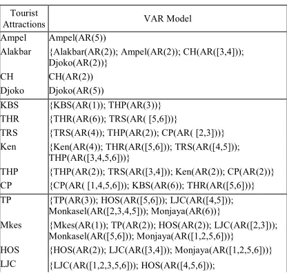
Output of VAR modeling to the tourists visit data is shown in Table 1. The second column of Table 1 shows VAR model. We see that Alakbar, as an example, has model of {Alakbar(AR(2)); Ampel(AR(2)); CH(AR([3,4])); Djoko(AR(2))}. It means that the number of tourists visiting to Alakbar is influenced by the number of tourists visiting to: (i) Alakbar itself on lag 1 and lag 2 or written as Alakbar(AR(2)), (ii) Ampel on lags 1 and 2 or written as Ampel(AR(2)), (iii) CH on subset of lag 3 and of lag 4 or written as CH(AR([3,4])), and (iv) Djoko on lags 1 and 2 or written as Djoko(AR(2)).

Table 1: VAR model for each tourist attraction

Tourist

Attractions VAR Model

Ampel Ampel(AR(5))

Alakbar {Alakbar(AR(2)); Ampel(AR(2)); CH(AR([3,4])); Djoko(AR(2))}

CH CH(AR(2))

Djoko Djoko(AR(5))

KBS {KBS(AR(1)); THP(AR(3))} THR {THR(AR(6)); TRS(AR( [5,6]))}

TRS {TRS(AR(4)); THP(AR(2)); CP(AR( [2,3]))} Ken {Ken(AR(4)); THR(AR([5,6])); TRS(AR([4,5]));

THP(AR([3,4,5,6]))}

THP {THP(AR(2)); TRS(AR([3,4])); Ken(AR(2)); CP(AR(2))} CP {CP(AR( [1,4,5,6])); KBS(AR(6)); THR(AR([5,6]))} TP {TP(AR(3)); HOS(AR([5,6])); LJC(AR([4,5]));

Monkasel(AR([2,3,4,5])); Monjaya(AR(6))}

Mkes {Mkes(AR(1)); TP(AR(2)); HOS(AR(2)); LJC(AR([2,3])); Monkasel(AR([5,6])); Monjaya(AR([1,2,5,6]))} HOS {HOS(AR(2)); LJC(AR([3,4])); Monjaya(AR([1,2,5,6]))} LJC {LJC(AR([1,2,3,5,6])); HOS(AR([4,5,6]));

Monkasel(AR([3,4,5,6])); Monjaya(AR([3,4,5]))} Monkasel {Monkasel(AR(6)); HOS(AR([2,3,4,5])); LJC(AR(5));

Monjaya(AR(2))}

Monjaya {Monjaya(AR([1,3,4])); Mkes(AR([4,5,6])); HOS(AR([4,5,6])); LJC(AR(2)); Monkasel(AR([3,4]))} DRS {DRS(AR([4])); WRS(AR([4,5]))}

WRS {WRS(AR(3)); DRS(AR(1))}

Pres Pres(AR(2))

BP BP(AR(4))

The performance of the VAR model can be measured by employing MAPE of the VAR forecast and out-sample data. The MAPE value for each model is shown in Table 2. The smaller MAPE value mean the better forecast will be obtained. MAPE of VAR for WRS looks very bad. Besides there are only two variables influenced in the VAR of WRS, this can be caused by the variability of the number of DRS visitors is very big different with the number of WRS visitors, especially for the last period data which are used for calculating its MAPE.

3.2 Neural Network Modeling

Modeling with NN in this study will use

multilayer networks with backpropagation

ISSN: 1992-8645 www.jatit.org E-ISSN: 1817-3195 Table 2: MAPE value of VAR for each tourist attractions

Tourist Attractions MAPE

Ampel 31,99%

Alakbar 29,46%

CH 33,97%

Djoko 61,25%

KBS 68,06%

THR 37,89%

TRS 90,73%

Ken 4,57%

THP 72,05%

CP 86,64%

TP 39,43%

Mkes 33,11%

HOS 13,58%

LJC 31,24%

Monkasel 69,97%

Monjaya 114,02%

DRS 359,61%

WRS 1563,25%

Pres 16,40%

BP 906,83%

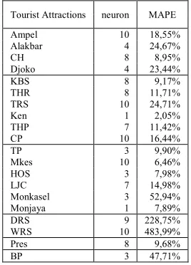
Table 3: The optimal number of neuron in hidden layer of NN for each tourist attractions

Tourist Attractions neuron MAPE

Ampel 10 18,55%

Alakbar 4 24,67%

CH 8 8,95%

Djoko 4 23,44%

KBS 8 9,17%

THR 8 11,71%

TRS 10 24,71%

Ken 1 2,05%

THP 7 11,42%

CP 10 16,44%

TP 3 9,90%

Mkes 10 6,46%

HOS 3 7,98%

LJC 7 14,98%

Monkasel 3 52,94%

Monjaya 1 7,89%

DRS 9 228,75%

WRS 10 483,99%

Pres 8 9,68%

BP 3 47,71%

The optimal number of neurons in each layer of NN model for each tourist attractions is shown in second

column of

Table 4. This column inform the structure of number of neurons in input layer, hidden layer, and output layer. The structure of NN model of Alakbar has the form of NN(8,4,1), which can be shown as Figure 3. Its mean that there are 8 neurons from 4

variables ( represents Ampel contributing 2

neurons, that are , and , , represents

Alakbar contributing 2 neurons, that are ,

and , , represents CH contributing 2

neurons, that are , and , , represents

Djoko contributing 2 neurons, that are , and

, ) in input layer, 4 neurons in hidden layer,

and 1 neuron in output layer.

Table 4: NN model

Tourist Attractions model

Ampel 5,10,1

Alakbar 8,4,1

CH 2,8,1

Djoko 5,4,1

KBS 4,8,1

THR 8,8,1

TRS 8,10,1

Ken 12,1,1

THP 8,7,1

CP 12,10,1

TP 17,3,1

Mkes 13,10,1

HOS 8,3,1

LJC 15,7,1

Monkasel 17,3,1

Monjaya 13,1,1

DRS 3,9,1

WRS 4,10,1

Pres 2,8,1

BP 4,3,1

Figure 3: NN architecture for Alakbar, NN(8,4,1)

The best VAR-NN for each tourist attractions can be illustrated graphically as a figure which is able to explain all multivariate relationship among tourist attractions. The graphical relationship for each of six groups of themes are

a. Religious Tourism

ISSN: 1992-8645 www.jatit.org E-ISSN: 1817-3195

Figure 4: Multivariate relationship among tourist attractions in group of religious tourism

b. Environment Tourism

Figure 5 shows the multivariate relationship among variables in environment tourism group theme. This figure demonstrates a relatively more complex multivariate relationship than in religious tourism network, Figure 4. In this group theme, each tourist attractions influenced not only by itself, but also by the others, that is: (1) KBS influenced by THP, (2) THR influenced by TRS, (3) TRS influenced by THP, and CP, (4) Ken influenced by THR, TRS, and THP, (5) THP influenced by TRS, Ken, and CP, (6) CP influenced by KBS, and THR. It can be said that tourists who visit one tourist attraction could be possibly also visit other tourist attractions in this group theme.

Figure 5: Multivariate relationship among tourist attractions in group of environment tourism

c. Museum & Monument Tourism

Figure 6 shows the multivariate relationship among variables in museum & monument tourism group theme. This figure represents the most complex multivariate relationship among all group themes. Each member of tourist attraction in this group theme is influenced by itself and any other tourist attractions, i.e. (1) TP influenced by HOS, LJC, Monkasel, and Monjaya, (2) MKes influenced by TP, HOS, LJC, Monkasel, and Monjaya, (3) HOS influenced by LJC, and Monjaya, (4) LJC

influenced by HOS, Monkasel, and Monjaya, (5) Monkasel influenced by HOS, LJC, and Monjaya, (6) Monjaya influenced by MKes, HOS, LJC, and Monkasel. It means that the number of tourists visiting in one tourist attraction influence by the number of tourists visiting in any other tourist attractions.

Figure 6: Multivariate relationship among tourist attractions in group of museum & monument tourism

d. Grave Tourism

Figure 7 shows the multivariate relationship between variables in grave tourism group theme. The figure shows that DRS and WRS influenced by each other. In other word, it means that the number of tourists in DRS influenced by number of tourists

inWRS and vice versa.

Figure 7: Multivariate relationship among tourist attractions in group of grave tourism

e. City Park Tourism

Because in this group only contain one tourist attraction, then the variable only influenced by itself, as shown in Figure 8.

Figure 8: Multivariate relationship in the group of city park tourism

f. Heritage Tourism

This last two group themes, heritage and city park tourisms, have the simplest model of tourism network. This heritage group is also containing only one tourist attraction as in city park tourism group theme. Therefore, the variable is also only influenced by itself, as shown in Figure 9.

Ampel

Z1

Alakbar

Z2

CH

Z3 Djoko

Z4

KBS

Z1

THR

Z2

TRS

Z3

Ken

Z4 CP

Z6

THP

Z5

TP

Z1

MKes

Z2

HOS

Z3

LJC

Z4 Monjaya

Z6

Monkasel

Z5

WRS

Z2

DRS

Z1

Pres

ISSN: 1992-8645 www.jatit.org E-ISSN: 1817-3195

Figure 9: Multivariate relationship in the group of heritage tourism

3.3 Model Comparison

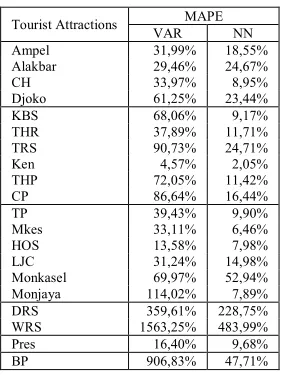
All models obtained by VAR method and NN are compared based on their MAPE. MAPE of VAR and NN for each tourist attractions are shown in Table 5. Based on this table, all of MAPE values of NN for each tourist attraction are smaller than of VAR method. This is because the NN has the ability to solve the nonlinear problems which is possibly containing in the data, and NN also able to model the complex relationships between inputs and outputs to capture the patterns in the data.

The different between MAPE value of VAR and NN is primarily influenced by the number of inputs used in the NN. NN which use more than one variables input, its MAPE will tend to decrease less than NN with one input variable.

Table 5: Comparison MAPE value between VAR and NN

Tourist Attractions MAPE

VAR NN

Ampel 31,99% 18,55%

Alakbar 29,46% 24,67%

CH 33,97% 8,95%

Djoko 61,25% 23,44%

KBS 68,06% 9,17%

THR 37,89% 11,71%

TRS 90,73% 24,71%

Ken 4,57% 2,05%

THP 72,05% 11,42%

CP 86,64% 16,44%

TP 39,43% 9,90%

Mkes 33,11% 6,46%

HOS 13,58% 7,98%

LJC 31,24% 14,98%

Monkasel 69,97% 52,94%

Monjaya 114,02% 7,89%

DRS 359,61% 228,75%

WRS 1563,25% 483,99%

Pres 16,40% 9,68%

BP 906,83% 47,71%

4. CONCLUSIONS

This paper has succeeded to demonstrate the work of NN in improving the accuracy of VAR modeling based on the minimum of MAPE. We also found the correlation among tourist attractions, but we cannot get the order of tourist arrival because it need use another method. Also the increasing number of neurons in the hidden layer does not always give effect to the decreasing the value of MAPE.

In this study, the data used is the monthly data. For further research, firstly it is recommended to get the data with a shorter time period, i.e. weekly

or even daily. Not only, it would be expected to give better results, but also the model could give a realistic movement of tourists from one tourism object to the other in order to estimate the number of city bus needed and their travel schedule. Secondly, this case can be analyzed using Bayesian Networks.

5. ACKNOWLEDGEMENT

We would like to thank to Surabaya Culture and Tourism Department which allow us to get the data of number of tourist visit in Surabaya tourist attractions. We thank also to blind anonym reviewers who give some advice and criticism to make this paper better.

REFERENCES

[1] H. Akaike, "A New Look at the Statistical

Model Identification," IEEE Transactions on

Automatic Control , vol. 19, no. 6, pp.

716-723, 1974.

[2] N. Y. Zainun, I. A. Rahman and M. Eftekhari, "Forecasting Low-cost Housing Demand In An Urban Area In Malaysia Using Artificial

Neural Networks: Batu Pahat, Johor," WIT

Transactions on Ecology and the Environment,

vol. 142, 2010.

[3] W. W. Wei, Time Series Analysis: Univariate and Multivariate Methods, 2nd ed., New York: Pearson Education, Inc, 2006.

[4] S. Haykin, Neural Networks: A

Comprehensive Foundation, New York:

MacMillan Publishing Company, 1994. [5] C. Gershenson, Artificial Neural Networks for

Beginners, New York: Cornell University Library, 2003.

[6] S. Kusumadewi, Artificial Intelligence (Teknik dan Aplikasinya), Yogyakarta: Graha Ilmu, 2003.

[7] P.-C. Chen, "Integrating Fuzzy Theory, Genetic Algorithm and Neural Network in

Tourism Forecasting," Advances in

information Sciences and Service

Sciences(AISS), vol. 5, no. 3, pp. 767-775,

2013.

[8] C.-J. Lin, H.-F. Chen and T.-S. Lee, "Forecasting Tourism Demand Using Time Series, Artificial Neural Networks and Multivariate Adaptive Regression Splines:

Evidence from Taiwan," International Journal

of Business Administration, vol. 2, no. 2, pp.

14-24, 2011.

[9] M. Khashei, S. R. Hejazi and M. Bijari, "A New Hybrid Artificial Neural Networks and Fuzzy Regression Model for Time Series

BP

ISSN: 1992-8645 www.jatit.org E-ISSN: 1817-3195

Forecasting," Fuzzy Sets and Systems, vol.

159, p. 769–786, 2008.

[10] A. Palmer, J. J. Montano and A. Sese, "Designing an Artificial Neural Network for

Forecasting Tourism Time Series," Tourism

Management , vol. 27, p. 781–790, 2006.

[11] Statistics of Surabaya City, Surabaya Dalam Angka, Surabaya: Statistics of Surabaya City, 2015.

[12] Secretariat of Surabaya Culture and Tourism Department, Direktori Pariwisata Surabaya 2014, Surabaya: Surabaya Culture and Tourism Department, 2014.

[13] P. Kumar, M. Murthy, D.Eashwar and M.Venkatdas, "Time Series Modeling Using Artificial Neural," Journal of Theoretical and

Applied Information Technology (JATIT), vol.

4, no. 12, pp. 1259-1264, 2008.

[14] S. N. Mandal, J. Choudhury, S. Chaudhuri and D. De, "Soft Computing Approach in Prediction of a Time," Journal of Theoretical and Applied Information Technology (JATIT),

vol. 4, no. 12, pp. 1131-1141, 2008.

[15] H. Song and G. Li, "Tourism Demand Modelling and Forecasting—A Review of

Recent Research," Tourism Management, vol.

29, p. 203–220, 2008.

[16] O. Claveria, E. Monte and S. Torra, "Tourism Demand Forecasting With Different Neural Networks Models," IREA Working Papers, Barcelona, 2013.

[17] O. Claveria, E. Monte and S. Torra, "A Multivariate Neural Network Approach To

Tourism Demand Forecasting," IREA