3644
ALGEBRA FOR TRANSFORMING THE STRUCTURE OF
THE SEARCH SPACES ASSOCIATED WITH THE
COMBINATORIAL OPTIMIZATION PROBLEMS
ARTEM POTEBNIA
Alumnus, Kyiv National Taras Shevchenko University, Ukraine; ORCID: 0000-0002-8162-5613;
Website: artem.pp.ua; E-mail: [email protected]
ABSTRACT
This article proposes the classification of the search spaces associated with the combinatorial optimization problems based on the type of their constituent solutions. The spaces belonging to each identified class are accompanied by the corresponding graph models. Against this background, the article introduces the original algebra allowing the representation of the search spaces in the unified homogeneous form. The proposed algebra consists of a set of transformations given in an analytical form and illustrated by the modifications of the graph models constructed for the search spaces.
Keywords: Combinatorial Optimization Problem, Search Space, Bipartite Graph, Multigraph, Graph.
1. INTRODUCTION
Solving the combinatorial optimization problems constitutes the keystone of modeling and designing the computer-based information systems. For example, the problem of the VLSI circuits partitioning could be reduced to the problem of finding the cuts in hypergraphs [1]. In turn, the quality of its solving significantly affects the properties of the manufactured devices such as the energy consumption, delays, cost of producing, etc.
Similarly, the construction of the large-scale GRID and cloud computing infrastructures is inextricably linked with solving the tasks scheduling and load balancing problems in order to ensure the optimal usage of the available resources [2]. Another prime example is associated with scheduling packets in the wireless networks equipped with the relay nodes, which represents the variation of the multiple-choice multi-dimensional knapsack problem [3, 4].
At the same time, a number of the known combinatorial optimization problems formulated in the decision form are NP-complete [5, 6]. Due to the combinatorial explosion effect, the algorithms returning their exact solutions have the exponential time complexity, which underlies the inefficiency of their application to the large-scale problem instances. As a result, the efforts to solve such problems are intrinsically linked with the development of the metaheuristic algorithms aimed
to produce the approximate solutions in a reasonable time. The fundamental strategy followed by such algorithms lies in manipulating by the solutions in order to shrink the explored search space. Looking into more detail, the search process implemented by the metaheuristics is based on performing the iterative improvements of the single current solution (e.g. simulated annealing, guided local search, tabu search) or population of solutions (e.g. evolutionary algorithms) [7].
The implementations of these algorithms are extremely sensitive to the representation of the solutions comprising the search spaces associated with the instances of the problems. However, the natural form of solutions encoding is problem-specific, which sufficiently complicates processing and analyzing the corresponding search spaces [8]. For example, the solutions of the Boolean satisfiability problem could be easily encoded by the bit vectors indicating the values taken by the variables. On the contrary, the solutions of the traveling salesman problem naturally are represented by the permutations of the graph’s vertices [7, 9]. Notice that the form of solutions encoding is particularly acute when designing the adaptations of the metaheuristics for the specialized computer architectures such as the graphical processing units due to the need for managing the memory allocation [10].
3645 canonical way for representing the search spaces. However, for a number of problems such encoding requires performing the non-trivial transformations of the search spaces. Therefore, the objective of this article is to propose the algebra for transforming the structure of the search spaces to the unified homogeneous form.
2. CLASSIFICATION OF THE SEARCH
SPACES ASSOCIATED WITH THE COMBINATORIAL OPTIMIZATION PROBLEMS
The primary challenge in achieving the intended objective is that the well-known definitions of the combinatorial optimization problem [11, 12] are formulated without detailing the structure of the search spaces. Consequently, due to such insensitivity, these definitions could not be used as a basis for classifying the search spaces and their constituent solutions. This causes the need for introducing the new more detailed definition of the combinatorial optimization problem, which constitutes the first significant contribution of this article.
Definition 1. The combinatorial optimization problem is represented by a set of instances given in the form of pentuples I= , , , ,Pϕ Φ Ψ , where
denotes the finite (or countably infinite) search space associated with the particular instance. This space encompasses the combinatorial configurations X and is constructed by applying the generating combinatorial operator to the finite (or countably infinite) base set P=
{
p1,...,pn}
. Moreover, each instance I is equipped with the indicator function ϕ:→{ }
0,1 taking the value of 1 for all configurations X′∈ satisfying the constraints of the problem. The optimality of all elements X∈ is reflected by the family{
f1,...,fm}
Φ = of the objective functions :
i
f →R defined over the entire configuration space and the collection Ψ =
{
extr1,...,extrm}
of the optimization criterions extri ={
min,max}
for all functions fi.In the context of such formulation, the configurations X comprising the search space
represent all possible solutions of the problem instance I. Notice that according to Definition 1, the elements of both set P and space are isolated from each other. Obviously, there always exists the uncountable infinite set U P⊃ in which any
element p P∈ could be surrounded by the non-empty punctured neighborhood N p
( )
⊆U such that N p( )
P= ∅. The isolation of all configurations X∈ could be demonstrated in a similar manner. This clearly shows that Definition 1 does not cover the continuous optimization problems.Remark that by virtue of introducing the families of the functions Φ and criterions ,Ψ Definition 1 is sufficiently flexible to cover the multi-objective optimization problems. At the same time, in the simplest case of the single-objective problems, the families Φ and Ψ contain respectively just one function f and criterion extr, i.e. m=1. As a consequence, the instances of such problems could be represented in the simplified form
, , , , .
I= Pϕ f extr
Let us denote by ′ ⊆ the set of all feasible solutions satisfying the constraints of the problem instance I, i.e. ϕ ′ =
( )
1. Under such approach, the exact solution for the instance I of the single-objective problem takes the form of the configuration X0′ ∈ ′ such that the value f X( )
0′constitutes the global minimum or maximum (depending on the criterion extr) of the objective function f over the set ′. Notice that the instance of the combinatorial optimization problem might be deprived of the feasible solutions in the case of
. ′ = ∅
The generating combinatorial operator
ensures filling the configuration space with the structures implementing different forms of the relationship between the elements of the base set P
(such as the combinations, permutations, selections, etc.). Accordingly, the instances of the combinatorial optimization problems could be equipped with the configuration spaces of various types, which substantially differ in representing the elements X∈. In spite of the huge variety of possible concrete implementations of the operator, we can indicate four fundamental classes of the search spaces . Let us introduce the notations ( )i and X( )i for the spaces belonging to the i-th class and their constituent configurations. Remark that the search space ′( )i composed of the feasible solutions
( )i
3646 Looking into detail, the classification proposed in this article distinguishes the classes whose representatives are:
1. The spaces (1) whose elements are represented simply by the unordered sets
{
}
(1)
1,..., t
X = x x ⊆P deprived of the repeated elements.
2. The search spaces (2) composed of the multisets that allow the multiple occurrences of the constituent elements but are indistinguishable from the perspective of their order. The solutions contained in such spaces have the form of pairs X(2)= XU,θ including of the underlying ordinary set of elements XU⊆P associated with the multiplicity function θ:XU→N≥1. The image of any element p X∈ U under the function θ reflects the number of all its occurrences in the configurationX(2).
3. The search spaces (3) comprised of the chains that are sensitive to the order of the elements but do not presuppose their duplications. In this case, each configuration is given by the set XU ⊆P paired with the function δ:XU →
{
1,2,...,XU}
reflectingthe order of elements, i.e. X(3)= XU, .δ In particular, δ
( )
p =t shows that the elementU
p X∈ occupies the t-th position in the solution X(3).
4. The spaces (4) whose elements are represented in the most sophisticated form of the “ordered multisets” encapsulating the information about the order of the elements that could be repeated. In turn, the solutions comprising such spaces could be represented by quadruples X(4)= H X, U, ,θ λ , where H
denotes the auxiliary set equipped with the function λ:H→
{
1,2,...,H}
specifying the order of its elements. On the other hand, the set H is constructed from the underlying setU
X and function θ:XU→N≥1 in the following way:
( )
{
1,..., i}
.i U
p i i p X
H p pθ
∈
=
For example, the instances of the 0-1 knapsack problem are generated from the base sets P
composed of n items associated with the prescribed values of the weight w p
( )
and cost c p( )
. These instances are equipped with the configuration spaces (1) that include 2n unordered sets(1)
X ⊆P reflecting all possible variants of packing the knapsack represented as the combinations of the items p P∈ produced by the operator . Obviously, such spaces belong to the first class according to the proposed classification. The limitation of the maximum load capacity of the packaged knapsack Q is taken into account by the function ϕ that outputs the value of 1 only for the configurations X′(1) satisfying the following condition:
( )
(1) .
p X
w p Q
′ ∈
≤
∑
In turn, the pursuit of packing the knapsack with the most valuable items leads to introducing the criterion extr=max and specifying the next objective function:
( )
( )
(1)
(1) .
p X
f X c p
′ ∈
′ =
∑
For contrast, let us consider the modified version of this problem that allows adding the multiple copies of any item to the knapsack. Its instances are equipped with the search spaces (2) of the second class, while their constituent configurations X(2) are the multisets representing the combinations of the elements p P∈ with repetitions.
It is noteworthy that some combinatorial optimization problems exhibit several natural schemes of generating the instances equipped with the search spaces of different classes. A prime example is the traveling salesman problem for the graph G=
(
V E,)
whose instances could be associated with the third class space (3)composed of the configurations X(3) reflecting the permutations of the vertex set V that serves as the base set. However, this problem could be characterized by the alternative set of instances having the first class spaces (1) comprising the V -combinations of the edges e E∈ . In this case, the base set is represented by the collection of edges E.
3647 multiple visits of each node v V∈ . The instances of such problem could be equipped with the fourth class spaces (4) whose elements X(4) represent the permutations with repetitions of the set V. The alternative way involves the formation of the instances accompanied by the second class spaces
(2)
including the combinations with repetitions of the edges e E∈ . These examples clearly insinuate the possibility of transforming the search spaces, which is discussed more fully in the remainder of this article.
3. REPRESENTATION OF THE SEARCH
SPACES BY THE GRAPH STRUCTURES
Since according to Definition 1 all solutions are constructed from the elements of the base set, the structural organization of the search space could be described in the form of the undirected bipartite graph S
( ) (
= V V EP X, , PX)
. The vertices of its first part vP∈VP are in line with the elements of the base set P, while the nodes of the second partX X
v ∈V embody the configurations X∈. Notice that the forbidden solutions belonging to
′
are ignored in the structure of the graphs
( )
S , which ensures considering the problem constraints. Moreover, each vertex vX ∈VX is equipped with m weight coefficients reflecting the values of the weight functions
{
f1,...,fm}
for the corresponding configuration X. In turn, the collection (set or multiset depending on the class of the modeled space ) EPX contains the edges connecting the nodes that belong to the different parts of the graph S( )
. In particular, each edge(
v vkP X, j)
∈EPX reflects the inclusion of the base set element pk in the configuration Xj.Taking into account the classification of the configuration spaces proposed in the previous section, we should emphasize that the type of the graph S
( )
significantly depends on the class of both spaces and ′. In particular, the first class spaces (1) are represented by the simple (i.e. deprived of the parallel edges) graphs S( )
(1) . On the contrary, the search spaces (2) of the second class are described in the form of the multigraphs( )
(2) .S Their multisets EPX include the parallel edges that are needed for reflecting the repeated entries of the base set elements in the configurations. For the third class spaces (3), the graphs S
( )
(3) are simple but additionally equipped with the weight function defined over the set of edges EPX. The value of this function for each edge(
v vkP X, j)
reflects the position of the base set element pk in the solution X(3)j and equals( )
pk .δ The fourth class spaces (4) constitute the most complicated case for representing and are reflected by the multigraphs S
( )
(4) with the weight function defined over the multisets of edges. PX E
4. OPERATIONS FOR UNIFICATION AND
HOMOGENIZATION OF THE SEARCH SPACES STRUCTURE
In summing up the previous section, the search spaces of the first class are the most convenient for the analysis and representation in terms of the graph structures. This underlines the desirability of converting the spaces (2), (3), and (4) into the equivalent first class spaces.
Definition 2. The operation of the search space unification involves representing the problem instances I= ( )i , , , ,Pϕ Φ Ψ for which
{
2,3,4}
i∈ in the new form
(1), , , , .
I∗= ∗ P∗ϕ∗ Φ Ψ∗ Accordingly, all search spaces belonging to the first class are referred as having the unified structure.
This operation could be reduced to implementing the transformations iP,iX such that
( )
P
i P =P∗
and iX
( )
X( )i =X∗(1). Here the transformation iP ensures translating the base set, while iX converts all possible configurations.3648 (1)
∗
is obtained simply by substituting all configurations X( )i ∈( )i with the corresponding outputs iX
( )
X( )i . The family of criterions Ψremains unchanged under the unification, while the functions f∗∈Φ∗ and ϕ∗ are defined on the new domain ∗(1). Let us represent the function ϕ by the set of pairs
(
X( )i ,ϕ( )
X( )i)
. Under this representation, the function ϕ∗ could be constructed by replacing these pairs with the modified ones(
iX( ) ( )
X( )i ,ϕ X( )i)
. Moreover, the objective functions f∗∈Φ∗ could be formed in the similar manner.Obviously, the unification does not affect the cardinality of the search space, i.e. ( )i = ∗(1) . Notice that the transformations iP and iX are applied only to the base sets and configurations of problem instances equipped with the search spaces belonging to the i-th class.
The transformation 2P translates the initial base set P into the following one:
( )
1 22
1
,..., i ,
n
m P
i i i
P p p
=
=
where n denotes the cardinality of the set P, while 2
i
m is the maximum value of θ
( )
pi among all configurations X(2)∈(2). Notice that the set( )
2P P holds
∑
in=1(
mi2−1)
more elements than the initial set P. In turn, the transformation 2Xensures representing each concrete configuration
(2) ,
U
X = X θ in the next form:
( )
(2){
1 ( )}
2 ,..., i .
i U
p X
i i p X
X p pθ
∈
=
In simple terms, any element pik∈2P
( )
Pcorresponds to the k-th copy of the element p Pi∈
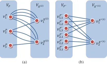
appearing in the solutions X(2)∈(2). Fig. 1a shows the simplified example of the second class search space (2) represented by the multigraph structure S
( )
(2) . In this case, the base set includes the elements p1, p2, and p3, while thespace (2) encompasses two solutions X1(2) and (2)
2
X . For example, the configuration X1(2) is composed of the element p2 and three copies of the element p1. As is evident from Fig. 1a, the existence of n copies of the base set element in one configuration is reflected in the corresponding multigraph by the “dipole” structure composed of n
parallel edges.
The result of performing the unification of this space is presented in Fig. 1b. Notice that the vertices vi kP,∗ correspond to the elements pik of the base set 2P
( )
P . The representation of all copies of the elements p Pi∈ by the separate elements (distinguished by the index k) in the set 2P( )
P [image:5.612.314.521.346.470.2]leads to the elimination of all parallel edges in the corresponding graph structure. Therefore, the resulting graph given in Fig. 1b is simple.
Figure 1: Graph Structures Representing the Sample of the Second Class Search Space (a) and the Result of
Implementing the Operation of Its Unification (b)
On the contrary, the transformation 3P produces the following output set:
( )
1 33
1
,..., i ,
n
m P
i i i
P p p
=
=
where mi3 is the maximum cardinality of the underlying set XU such that pi∈XU among all solutions X(3)∈( )3 . Similarly to the previous case, the cardinality of the resulting set 3P
( )
P is larger by∑
ni=1(
mi3−1)
compared to the initial setP. At the same time, the appropriate transformation 3X
translates the argument configurations
(3) ,
U
3649
( )
(3){ }
( )3 i .
i U
p X
i p X
X pδ
∈
=
In short, each element pik∈3P
( )
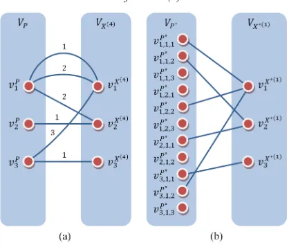
P corresponds to the element p Pi∈ contained in the configurations X(3)∈( )3 at the k-th position. Fig. 2a depicts the example of the third class search space (3). Its structure is illustrated by the graph( )
(3)S whose edges are accompanied with the weight coefficients reflecting the values of the function δ. In particular, the configuration X1(3)
includes the elements p1 and p2 located respectively at the first and second positions. Fig. 2b presents the structure of the search space obtained after implementing the operation of the unification. The more close inspection shows that the information encoded by the weight coefficients in Fig. 2a is expressed in Fig. 2b by the index k of the vertices vi kP,∗ representing the elements
( )
3 .
k P i
p ∈ P
At the same time, the formation of the base sets representing the outputs of the transformation 4P
involves the appropriate consideration of both ordering and repeating of the elements in the configurations X(4)∈( )4 . Thus, the expression for the sets 4P
( )
P takes the following complicated form:( )
,1 , 44 ,..., i ,
k
i H
k m
P k
i i
p P
P p p ′
∗
∈
=
where mi4′ is the maximum value of
( )
Up X∈ θ p
∑
among all configurations X(4) such that pi∈XU. In turn, the set PH∗ is defined as follows:
4
1 1
,..., i ,
n
m
H i i
i
P∗ p p
=
=
where mi4 denotes the maximum value of θ
( )
pi among all configurations X(4)∈( )4 .The presence of the auxiliary set H in the structure of the tuples X(4)= H X, U, ,θ λ
provides the opportunity to present the expressions for the outputs produced by the transformation 4X
in the next simple form:
( )
(4) ,( )
4 .
k i
k i
k p X
i p H
X p λ
∈
=
Thus, the unification of the fourth class search spaces requires the combination of the techniques used for unifying the second and third class spaces. The example of implementing such operation is shown in Fig. 3. Remark that the nodes vi k lP, ,
∗
[image:6.612.313.522.406.583.2]of the resulting graph reflect the elements pik l, of the base set 4P
( )
P .Figure 2: Structure of the Sample Third Class Search Space (a) and Its Modification in the Process of the
Unification (b)
Figure 3: Graph Models Constructed for the Instance of the Fourth Class Search Space (a) and Its Unified
Variant (b)
3650 different number of edges e E∈ . In order to deal with such situations, this article introduces the following operation:
Definition 3. The operation of the search space homogenization is applied to the problem instances
(1), , , ,
I = Pϕ Φ Ψ having at least two solutions (1), (1) (1)
j k
X X ∈ such that Xk(1) ≠ X(1)j and consists in their transition to the new form
(1)
ˆ ˆ ,ˆ,ˆ, ,ˆ
I = Pϕ Φ Ψ in which all solutions (1) ˆ(1)
ˆ
X ∈ have the equal cardinality. The search spaces are referred as having the homogeneous structure if they have the unified structure and encompass only the configurations having the equal cardinality.
Similarly to the previous case, the implementation of this operation comes down to specifying the pair of transformations ˆP,ˆX such that
( )
ˆP P =Pˆ
and ˆX
( )
X(1) =Xˆ(1). These transformations are given by the following expressions:( )
{
0 1}
1ˆP n , ,
i i i
P p p
=
=
( ) {
(1) 1 (1)} {
0 (1)}
ˆX .
i i i i
X = p p X∈
p p X∉
In simple terms, the transformation ˆP
( )
Pperforms “splitting” each element p Pi∈ into the pair of the new elements
{
p pi0 1, i}
. In turn, the configurations ˆX( )
X(1) are required to include exactly one element from each such pair, which clearly shows the equalization of their cardinality. [image:7.612.315.522.72.316.2]
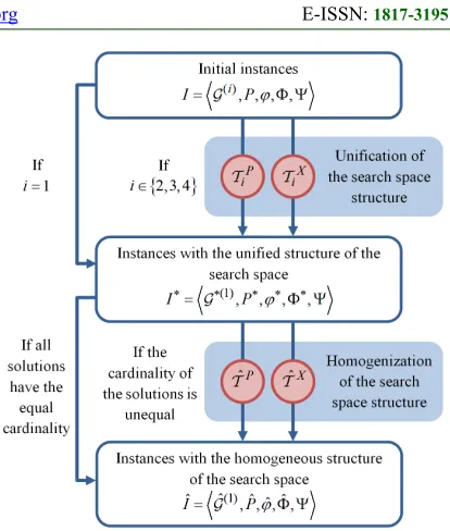
Figure 4: Graph Models Demonstrating the Structure of the Sample First Class Search Space Before (a) and After
(b) Performing Its Homogenization
Figure 5: Diagram Illustrating the Main Stages of Transforming the Problem Instances in Order to Construct the Search Spaces Having the Unified
Homogeneous Structure
Fig. 4 depicts the example of the search space homogenization. In particular, the graph model constructed for the initial non-homogeneous space (Fig. 4a) includes the vertices v1X(1) and v2X(1) reflecting the solutions X1(1), X2(1)∈(1) and having the degrees of 3 and 1, respectively. On the contrary, the nodes v1Xˆ(1) and v2Xˆ(1) of the graph given in Fig. 4b represent the configurations formed after performing the homogenization of the search space. Note that both these nodes have four adjacent vertices vi kP,ˆ corresponding to the elements pik of the base set ˆP
( )
P , which clearly illustrates the effect of the homogenization.Obviously, the application of the transformation
( )
ˆP P
[image:7.612.91.299.554.692.2]3651
5. CONCLUSIONS
As shown in Fig. 5, the fundamental idea of the proposed algebra lies in performing two operations modifying the structure of the search spaces associated with the problem instances. In particular, the operation of the unification results in blurring the class-based differentiation of the search spaces. It is followed by the operation of the homogenization intended to equalize the cardinality of all possible solutions.
As a result, the search spaces passed through both stages of transformation are eligible for encoding by the sets of the equal-length strings drawn from the binary alphabet. Under such encoding, the elements of the base set included in any solution could be indicated by ones in the corresponding string. At the same time, the opportunity to present the structure of the search spaces in the unified homogeneous form afforded by the proposed algebra has the drawback expressed by increasing the cardinality of the base sets.
REFERENCES
[1] W. K. Mak and D. F. Wong, “A Fast Hypergraph Min-Cut Algorithm for Circuit Partitioning”, Integration, the VLSI Journal, Vol. 30(1), 2000, pp. 1 – 11.
[2] Y. Fan, Q. Liang, Y. Chen, X. Yan, C. Hu, H. Yao, C. Liu, and D. Zeng, “Executing Time and Cost-Aware Task Scheduling in Hybrid Cloud Using a Modified DE Algorithm”,
Computational Intelligence and Intelligent Systems. Communications in Computer and Information Science, Vol. 575, 2016, pp. 74 – 83.
[3] R. Cohen and G. Grebla, “Multidimensional OFDMA Scheduling in a Wireless Network With Relay Nodes”, IEEE/ACM Transactions on Networking, Vol. 23(6), 2015, pp. 1765 – 1776.
[4] H. Kellerer, U. Pferschy, and D. Pisinger. “Knapsack Problems”, Springer, 2004
[5] A. Potebnia, “Method for Classification of the Computational Problems on the Basis of the Multifractal Division of the Complexity Classes”, Proceedings of the Third International Scientific-Practical Conference on Problems of Infocommunications. Science and Technology (PIC S&T), 2016, pp. 1 – 4. [6] A. Potebnia, “Representation of the Greedy
Algorithms Applicability for Solving the Combinatorial Optimization Problems Based
on the Hypergraph Mathematical Structure”,
Proceedings of the 14th International Conference on The Experience of Designing and Application of CAD Systems in Microelectronics (CADSM), 2017, pp. 328 – 332.
[7] R. Franz, “Design of Modern Heuristics: Principles and Application”, Springer-Verlag Berlin Heidelberg, 2011.
[8] C. Reidys and P. Stadler, “Combinatorial Landscapes”, SIAM REVIEW, Vol. 44, 2002, pp. 3 – 54.
[9] A. K. Kamrani and E. A. Nasr, “Engineering Design and Rapid Prototyping”, Springer US, 2010.
[10]T. Van Luong, N. Melab, E.G. Talbi, “GPU Computing for Parallel Local Search Metaheuristic Algorithms”, IEEE Transactions on Computers, Vol. 62(1), 2013, pp. 173 – 185. [11]E. Aarts and J. K. Lenstra, “Local Search in
Combinatorial Optimization”, John Wiley & Sons Ltd., 1997.