2402
USING DRIFT INTENSITY AS A BASIS FOR HANDLING
CONCEPT DRIFT IN CLASSIFICATION SYSTEMS
1HISHAM OGBAH, 2ABDALLAH ALASHQUR
1Faculty of Information Technology,
Applied Science University, Amman, Jordan
2Professor, Faculty of Information Technology
Middle East University, Amman, Jordan
Email: [email protected] , [email protected]
ABSTRACT
Concept drift is a known problem that can occur in classifier systems. Detecting and handling concept drift is an active area of research. Once a concept drift is detected, it has to be handled by updating or re-generating the classification model. In this paper, a new approach is introduced for handling concept drift, where a drift intensity measure is used to quantify the intensity of a concept drift. The model generation process uses the drift intensity measure while generating a new model. If the drift intensity is high, the model generation process discards old data (data before the drift occurrence) and builds a new model solely based on the new data after drift. On the other hand, if the drift intensity is low or moderate, the model generation process takes into account both old data and new data but it gives more weight (proportional to the drift intensity) to the new data as compared to old data.
Keywords: Data Mining,Classification, Concept Drift, Drift Handling, Big Data.
1. INTRODUCTION
In classification each tuple in a dataset is mapped to one of a limited set of classes. A specific column in the dataset is designated as the class label, in
which the class name of each tuple is stored [1,2,3,4,5,6]. The primary objective of a classifier is to be able to predict the classification of newly added tuples that have not yet been classified. This is usually accomplished by, first, going through a machine learning phase in which the system learns the classification model from a training dataset (i.e., a pre-classified dataset). After learning the classification model, the system is ready to go through the second phase in which it can predict the classification of new tuples [7,8].
A problem takes place if the distribution of data tuples with respect to classes changes after a period of time. Meaning that data tuples that used to legitimately map to, say, class1, now map to another class, say, class2. However, a system that learned the classification model prior to the change in data distribution will continue to predict class1 for the same piece of data, while in reality it should be class2. Thus a mismatch occurs between the system’s predictions and the actual classifications, which is referred to as concept drift [9,10,11]. If a
concept drift is not detected and dealt with properly, it results in producing inaccurate predictions. In this paper we introduce a new algorithm for handling a concept drift. It is based on the authors’ earlier work on detecting concept drift [6], where a way for quantifying and measuring the drift intesity (DI) was introduced. Further, based on the DI value, the intensity of a drift was categoriezed as either high, medium, or low.
The handling algorithm introduced in this paper generates a new classification model if a drift has been detected. It is different from existing algorithms in that the newly generated model is based on both data before drift as well as data after drift. However the weight given to data after drift by the algorithm is larger than the weight given to data before drift. Therefore data after drift has more influence on the new model generation process than data before drift.
2403 In the extreme case when the drift intensity is sever, the algorithm gives a weight of zero to the data before drift and full weight to the data after drift. In this case it generates a new classification model solely based on the data after the drift whereas the data before drift is totally ignored during the model generation process.
The user is given the ability to overwrite the algorithm’s default weights. For example, if the drift intensity is low, the algorithm will give some weight to data before drift. The user can overwrite this behavior and decide to give zero weigh to data before drift and full weight to data after drift, thus forcing the generation of a new model solely based on data after drift. This capability makes our new algorithm more generic in the sense that it can mimic the behavior of traditional concept drift algorithms, which totally ignore data before drift when generating a new classification model. The remainder of this paper is organized as follows. In Section 2 we provide a survey of related work. Section 3 presents the formulas used to compute the Drift Intensity. Section 4 describes the new algorithm used for handling concept drift. Section 5 explains decision tree algorithm and how to apply weight-based approach with classification algorithm. Implementation results are shown in Section 6. Finally, conclusions are given in Section 7.
2. RELATED WORK
Many adaptive algorithms used for learning use the most recent data as a basis for prediction because they assume such data to be most informative. Therefore, data management typically aims at learning from the most recent data. There are two types of training windows size: fixed or variable. Sliding window of a fixed size stores a
particular number of the most recent instances. When a new instance arrives, it is saved in the training window and the oldest one is thrown away. The sliding window of variable size, on the other
hand, varies the number of instances in a the window as time goes on depending on either the indications of a change detector, or after a certain timestamp. This approach uses heuristics to adjust the window size to the current extent of drift [12, 13]. Below is a brief description of some of the techniques and mechanisms that are used to handle the predictive models of evolving data.
The WINNOW [14] is a linear classifier that
uses an approach in which the trainer responds to each sample according to a certain hypothesis.
Based on the current classification of the example, the learner can updates the hypothesis. The main characteristic of WINNOW is its resilience to
irrelevant features [14]. WINNOW does not have
explicit forgetting techniques. Therefore, adaptation takes place mainly when the old concepts are diluted, because of the new arriving data. The WINNOW is capable of adapting itself to
slow drifts over time. Its main limitation is the slow adaption to the occurrence of sudden drifts. A tradeoff between stability and sensitivity is required for setting these parameters [10, 15].
The algorithm family FLORA [16] presents a
new approach in which the predictive model is kept consistent with a set of very recent instances. FLORA uses a sliding window of fixed size. It stores the most recent models on the basis of a first-in-fist-out (FIFO) approach. At each step the algorithm builds a new model based on instance selection from the training window that moves over recently arrived instances. The model is updated depending on two processes: a learning/selecting process, which updates the model based on the recent data. And a forgetting process that throws away data that is moved out of the window. The primary challenge in this approach is to determine an appropriate window size. In case of using a large window it gives a better performance in stable periods. But it responds to concept drifts in slower fashion. In case of using a short window, it mimics the current distribution more precisely. Therefore, it can guarantee fast adaptation as time goes on with concept drifts. But during stable period a very short window degrades the performance of the system [10, 17].
The FLORA2 [16] is one of the earliest
algorithms, that uses an varying window size. Adaptive window maintains the consistency of the predictive model with current concept. Upgraded versions of the algorithm have been improved to work with recurring concept such as FLORA3, and
noisy data FLORA4. Another study described in
2404 The author of [21] presents a new approach for gradual forgetting, that is applied to learn concept drift. The approach proposes the introduction of a time-based forgetting function, which makes the last instances observation more significant for the learning algorithms than the old ones. The advantage of time-based forgetting function that there are no instances are completely discarded from the training dataset. And, they are decreased with time. This approach provides each training instance with a weight that reflects their age, according its appearance over time. Instance weighting is based on an the assumption that the significance of an tuple in the training dataset must be decreased with as time goes on. This approach which is linear decrease approach can also be found in [22], and another technique that uses exponential decrease is published in [23].
In general, the existing approaches to cope up with the phenomenon of concept drift can be divided into two categories. First, approaches that adapt a model at regular intervals without considering whether drifts have really occurred or not, such as fixed or variable sliding window and weighted instances. When a sliding window is used, the model is created only from the instances; that are included in the window within a particular number of the most recent instances in fixed sliding window or within a certain time in variable sliding window. Besides forgetting all previous instances. The key point in this approach is how to select the appropriate window size. Whereas the idea of weighted instances is based on that the importance of instances should decrease with time according to their age and appearance. Second, approaches that first detect drifts, and then the model is adapted to these drifts. In order to detect concept drifts, the model is monitored over time. If a concept drift occurred, some procedures to adapt the model to these drift should be taken. For example, when a sliding window of variable size is used these procedures usually lead to decrease the window size according to the extent of concept drift. In both categories, none of them uses weight approach and gives more weight to the recent data, and gives less weight to the older data rather than discard them.
3. DRIFT INTENSITY (DI)
In this section, the drift intensity (DI) measure,
as introduced by the authors of this paper in [6], is summarized. DI is a metric used to measure the intensity of a drift in the underlying data with respect to their classes. The DI value provides a
measure of how sever the drift is. Furthermore, in this paper, we use the DI value to guide the concept drift handling process.
A set of mathematical equations were introduced in [6] to measure the DI value. Two sample subsets are taken from the dataset, one from before the drift location (DBD) and the other one from after the drift
location (DAD). It is assumed that DBD and DAD are
of equal size. Using sample subsets instead of the entire dataset enables us to avoid scanning the whole dataset, which degrades performance when dealing with big data sets. A reasonable size of each of DBD and DAD can be no more that 0.5% of
the dataset.
In the following, the error rate in predictions (i.e., the rate at which the predicted classes are inconsistent with the actual classes) in both subsets, DBD and DAD, is used as a way to measure the
intensity of a drift.
Let NBD and NAD be the number of data tuples in
DBD and in DAD, respectively. Also, let EBD and EAD
be the number of inaccurate classifications in DBD,
and DAD, respectively. Furthermore, let REBD and
READ be the classification error rates in DBD and
DAD, respectively. REBD and READ can be
calculated as follows.
RE E N 1
RE E N 2
The drift intensity can be computed by dividing the error rate before drift by the error rate after drift as shown in below.
DI RE
RE
However, because the resulting value of DI based on the above equation can be a very huge number, the above equation is modified as shown in Equation 3 by applying log2 in order to attenuate
the value of DI.
DI log RE
RE 3
Note that the denominator in Equation 3 (REBD)
becomes zero if EBD is zero. To avoid this zero,
Equation 1 is altered by adding “one” to the numerator as shown in Equation 4 below.
RE E 1
2405 In summary, to calculate DI we need to compute first the values of REBD and READ from Equations
4 and 2, respectively. Then we can substitute in Equation 3. An example of how to compute DI is shown below.
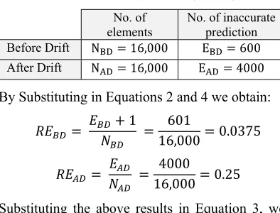
Example. Assume a certain dataset contains 3M tuples. Further assume a detection algorithm detects a drift in the third quarter of this dataset. The sizes of the sample subsets DBD and DAD are
16000 rows each (which is approximately 0.5% of the size of the dataset). Also, assume that the number of inaccurate classifications in DBD is NBD
= 600 and the number of inaccurate classifications in DAD is NAD = 4000. This combination of values
is summarized in Table 1.
Table 1: Errors Before And After Drift
No. of
elements No. of inaccurate prediction Before Drift N 16,000 E 600 After Drift N 16,000 E 4000 By Substituting in Equations 2 and 4 we obtain:
1 601
16,000 0.0375
4000
16,000 0.25
Substituting the above results in Equation 3, we obtain.
log log 6.66 2.736
3.1 DI Zones
The DI range of values is divided into three zones [6]. The low drift intensity zone ZL
represents values of DI in the range between 0.1 and 3, the medium intensity zone ZM represents
values of DI in the range between 3 and 6, and the high intensity zone ZH represents any values of DI
[image:4.612.91.288.294.444.2]greater than 6. Table 2 summarizes these zones.
Table 2: DI Zones
Zones DI value range Intensity of drift 0.1 – 3 Low drift intensity
3 - 6 Medium drift intensity Greater than 6 High drift intensity
4. CONCEPT DRIFT HANDLING
This chapter provides a description of a new handling algorithm called Weight-based Concept Drift Handling (WCDH) algorithm that we proposed for handling the phenomenon of concept drift in a dataset with class labels. The proposed WCDH algorithm introduces a new approach for handling concept drift depends on weight-based technique.
4.1 Overview of the WCDH Algorithm
The WCDH algorithm depends on the results that are found by the BCDD algorithm [6]. If the BCDD algorithm detects that there is a drift in the underlying data distribution, then the WCDH algorithm is called to handle the classification model depending on the DI value that was obtained from the BCDD algorithm. The following points distinguish WCDH algorithm from existing similar studies:
1) The WCDH algorithm gives the data in the underlying distribution dataset different weights according to their position (i.e., whether before or after the drift). While, the previous studies give all the data in the underlying dataset the same weight except the algorithm in [21], which decreases the weight of tuples gradually according to their age without considering whether a drift occurred or not. Therefore, the WCDH algorithm is different from other algorithms in detecting the drift and distributing the weight between old data and recent data according to the DI value.
2) The WCDH algorithm gives the data before drift less weight than the data after the drift. The change in weight is proportional to the DI value. This means that when building a new classification model it gives more significance to the data after drift and less significance to data before drift. While the previous studies either forget all the data before the drift and use only the data after the drift, or treat the old data the same as the recent data [19.20].
The WCDH algorithm will use the DI as a guidance and give the user advices as to how the concept drift should be handled. When the DI is in ZH, the system may choose to rebuild a new
2406 give more weight to data after drift and, at the same time, take into consideration data before the drift but give it less weight. That means the data after the drift will influence in the newly classification model more than it is influence by data before the drift.
The increase in the weight value after the drift point is proportional to the value of DI. Similarly the reduction of the weight value before the drift is proportional to the value of DI. Therefore, if the DI value is high, the weight of data after the drift can be high and continues to increase until it gives full weight for data after the drift and, in contrast, zero weight for data before the drift when the value of DI is very high. On the other hand, the user can overwrite the default weight generated by the WCDH algorithm and provide another weight value. Also, the user can discard the old data and only consider the recent data on the model generation process when the DI value in the high zone. And so, the WCDH algorithm will have behavior similar to previous algorithms.
This flexibility in determining the weight for data before drift and weight for data after drift gives satisfying results based on the user needs. It must be emphasized that the proposed approach does not consider all the historical data as a training set, but a sufficient subset of the dataset that was selected to compute the DI value.
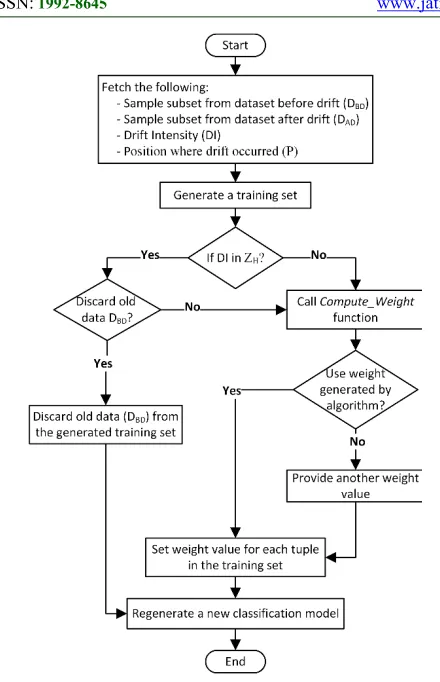
4.2 Flowchart and Pseudo Code of the Algorithm
Figure 1 shows the flowchart of the WCDH algorithm. At the beginning, the WCDH algorithm receives the following from the system: a sample subset of the dataset before drift (DBD), a sample
subset of the dataset after drift (DAD), drift intensity
(DI), and the position of drift (P) from the system.
After that, the training set is generated by concatenating the sample datasets DBD and DAD.
The algorithm checks the DI value, if the DI value is in ZH , the algorithm starts by giving the user the
option for discarding the old data or computing the weight for DBD and DAD . If the user selects to
discard DBD from the generated training set, the
algorithm discards DBD and goes to the final step,
which is re-generate a new classification model without DBD. On the other hand, if the user selects
to compute the weight for DBD and DAD or the DI
is not in ZH, the algorithm invokes
Compute_Weight function to compute weight for
DBD and DAD based on the formulas introduced in
Section 4.3.
After computing the weight for DAD andDAD the
algorithm gives the user the option to adjust the default weight value. Accepting the weight generated by the algorithm, the next step is to set weight for the generated training dataset. Otherwise, the algorithm allows the user to overwrite the default weight and then continue with processing weight for each tuple based on their position before or after the drift. The final step is to re-build a new classification model using any classification algorithm based on the weight assigned for tuples in data.
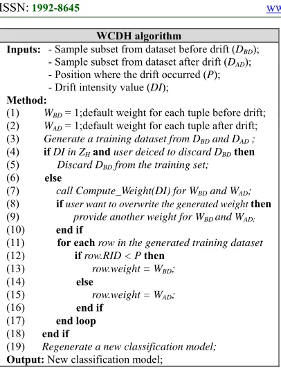
Figure 2 shows the pseudo-code of the WCDH algorithm. It works similar to the logic explained for the flowchart.
4.3 Compute_Weight Function
This section introduces the formulas that are used by WCDH algorithm to compute the weight of data before and after the drift. The weight is computed based on the DI value. The main processing of Compute_Weight function is to calculate the weight to be given to tuples. It gives more weight to data tuples after the drift and less weight to data tuples before the drift. The default if DI is in ZL or ZM is to use the weight computed
by the system. The user can modify that if he chooses. And, the default if DI is in ZH is to let the
2407 Figure 1: Flowchart of WCDH algorithm
2408 WCDH algorithm
Inputs: - Sample subset from dataset before drift (DBD);
- Sample subset from dataset after drift (DAD);
- Position where the drift occurred (P); - Drift intensity value (DI);
Method:
(1) WBD = 1;default weight for each tuple before drift;
(2) WAD = 1;default weight for each tuple after drift;
(3) Generate a training datasetfrom DBD and DAD ;
(4) ifDI in ZHand user deiced to discard DBDthen
(5) Discard DBD from the training set;
(6) else
(7) call Compute_Weight(DI) for WBD and WAD;
(8) if user want to overwrite the generated weight then (9) provide another weight for WBD and WAD;
(10) end if
(11) for eachrow in the generated training dataset
(12) ifrow.RID < Pthen
(13) row.weight = WBD;
(14) else
(15) row.weight = WAD;
(16) end if
(17) end loop
(18) end if
(19) Regenerate a new classification model;
[image:7.612.91.294.73.340.2]Output: New classification model;
Figure 2: Pseudo-code of the WCDH algorithm
In the following, a way to compute the weight based on DI is shown. The weight value is a function of DI. Let DIMin be the minimum value for
DI that is equal to 0.1. And, DIMax be either equal
to 10 in case of DI < 10 or take the same value as DI in case of DI ≥ 10. We assume that DIMax be as
DI value when DI ≥ 10 since the drift in this case is very high and is preferred to give zero weight for data before drift. In other words, DIMax can be
expressed as shown in Equation 6.
DI 10, orif DI 10
DI, otherwise 6
Let W∆ be the amount of change of the weight that
needs to be added or subtracted from the default weight given to tuple. To guarantee that W∆ is in
the range of 0 to 1 we use the following equation.
W∆
DI DI
DI DI 7
Let WBD be the weight of tuple before the drift, and
WAD be the weight of tuple after the drift. We
expect the value of WBD to be lower if we subtract
W∆ from the default weight. The formula for
calculating the value of WBD can be expressed as
shown in Equation 8.
W 1 W∆ 8
Also, we expect the value of WAD to be higher if
we add W∆ to the default weight. The formula for
calculating the value of WAD can be expressed as
shown in Equation 9.
W 1 W∆ 9
In conclusion, the value of WBD to be lower by
substituting in Equation 8, and the value of WAD to
be higher by substituting in Equation 9. The following subsection shows an example.
4.4 Example of Applying Compute_Weight
Function
In this example we will use the same sample subsets from dataset that we used in the example of applying DI equations. Where DI value is equal to 2.73 and the sample subsets of DBD and DAD that
forming the generated training is 16000 rows, each subset is 8000 rows.
For computing W∆, first determine the value of
DIMin and DIMax which they are equal to 0.1 and 10
respectively. DIMax is 10 since DI value is less than
10. Substituting in Equations 7, W∆ result is
obtained:
W∆
DI DI
DI DI
2.736 0.1
10 0.1 0.266
Substituting in Equations 8 and 9, the following results are obtained:
W 1 W∆ 1 0.266 0.734
W 1 W∆ 1 0.266 1.266
The weight for each tuple before the drift point in the training set is equal to 0.734 and the weight for each tuple from the drift point to the end of the training set is 1.266.
5. BUILD A NEW MODEL USING
WEIGHT-BASED APPROACH
2409 the analysis of the training dataset. A decision tree classification algorithm is one of the most popular classification algorithms in data mining [24,25] and it is applied in this paper to derive a new classification model. The following subsection describes the decision tree classification and shows how to apply the proposed weight-based approach with the decision tree for building a new classification model.
The decision tree represents an effective classification technique. It aims to split the training set into groups as possible in terms of the variable to be predicted. It takes as input a set of classified data (training set), and produces a tree that resembles a flowchart like tree structure, where each non-leaf node (internal node) represents a test on an attribute and each edge represents a result of the test. If the result of a test has two possible tuples belong to more than one class, further tests are required to complete the classification along that branch through adding more non-leaf nodes to the tree. Alternatively, if the outcome of a test consists of tuples that belong to the same class, then a leaf node is inserted to indicate that the tuples that satisfy the conjunction of the tests along the path from the root-node to the leaf-node are belong to only one class.
Various algorithms are available for constructing decision trees from training datasets such as: ID3 (Iterative Dichotomizer 3), C4.5, and CART (Classification and Regression Tree) [2, 4, 26]. There are many differences between these algorithms such as selecting certain attributes for splitting nodes in the tree.
In order to build a decision tree from training dataset an attribute selection measure is needed. The attribute selection measure is used to determine how the tuples at a given node are to be split. The attribute selection measure provides a ranking for each attribute representing the given training dataset. The attribute that have the highest score of the measure is selected as the splitting attribute for the given tuples.
Several common measures exist in the literature. In this paper a measure called Entropy (also called Information Gain) is used as one of those measures. This measure is used by ID3 for building decision trees [26]. At each node in the decision tree the attribute with the highest Entropy is selected as the splitting attribute. To find the attribute has the highest entropy, a three-step
proces is applied. Those steps are represented in the form of three equations 10, 11, and 12, that are explained as the following.
Step (1). Equation 10 is applied to compute the information needed to classify a tuple in the dataset , where is the class label, is the probability a tuple falls in the class.
log 10
Step (2). Equation 11 is applied to find the information required to classify the dataset based on the partitioning by . Each is a partition of the dataset , and | | is the number of the tuples in the partition.
| | 11
Step (3). In Equation 12 information gained by branching on attribute can be obtained by subtracting the result of Equation 11 from the result of Equation 10 as shown below.
12
Equation 10 is applied to the dataset only one time at the beginning. Equations 11 and 12 are applied for each attribute. The attribute that has the highest information gain is selected as the splitting attribute. This process is repeated at each level of the tree until leaf nodes are reached, which represent tuples that belong to only one class.
The contribution to improve decision tree is proposed by enabling the decision tree algorithm to support the weight-based approach. Indeed, when the result of a test belongs to different classes and no further splitting is possible, then decision tree selects a leaf node by choosing the most frequent class label. The integrating with proposed weight-based algorithm provides better solution for this issue, where a leaf node is selected by grouping the tuples that have same classes and using SUM function to compute the weight for each class. Then, selects the class that has the highest weight as a leaf node for the selected branch in the tree. The following subsections show how the decision tree with weight-based approach is built.
6. IMPLEMENTATION AND RESULTS
2410 new classification model. An experiment was conducted to evaluate the effectiveness of the WCDH algorithm with classification algorithm, and how the proposed approach achieves promising results. The model of the experiment is built using a decision tree algorithm. We use the first dataset that was used in evaluation the BCDD algorithm [6], which has one million row. Before conducting the experiment, let’s see how the model of the “Deals” dataset was been before it was injected with a drift. Figure 3 shows the decision tree model of Deals dataset.
The following are some notes about the xperiment we conducted:
1- The model was injected with a drift in the right branch in which “Age = 34–72” and goes through the edges identified by conditions “Gender = male”, and “Payment Method = credit card” ends up at the leaf node labeled with a “yes”. It is assumed that this path is changed to map class “no”.
2- The experiment show that the number of tuples before the drift point that map to class “yes” is 1400 and the number of tuples that was injected to map class "no" after the drift is 731.
3- After conducting the proposed approaches for detecting and handling concept drift the decision tree algorithm was called to build a new model.
The dataset was injected to contain a medium DI in ZM. After running the BCDD algorithm for
detecting the drift and measuring its intensity, the BCDD algorithm shows that the DI is 4.6. Then the WCDH algorithm was called to handle the drift by distributing the weight for each tuple in the generated training dataset based on its position before or after the drift. The WCDH algorithm shows that WBD is 0.546 and WAD is 1.454. After
that, the decision tree was invoked to build a new classification model.
As shown in Figure 4, the subtrees in which “Age > 34” was pruned since all the leaf nodes for that branch belong to the same class. The leaf node in which “Payment Method = credit card”, results to class “no”, because the weight of class “no” is higher than the weight of class “yes”, where weight of class “no” is 1063.2 and weight of class “yes” is 763.8 therefore this branch is mapped to class “no”. The two right branches in Figure 3 which “Age = 34-72” and “Age > 72” have been merged
to one branch in which “Age > 34” as shown in Figure 4 since they map to the same class.
From the above experiment it can be concluded that using the weight-based approach for generating a new classification model gives satisfying results. This is the same with what we expected since the weight-based approach will support a classification model to produce more accurate classification.
7. CONCLUSION
The occurrence of a concept drift in data is considered a problem that impacts the results of a classifier. A concept drift inhibits a classifier from generating accurate predictions because it results in making the classification model outdated if not totally obsolete. It is important to be able to detect and handle a concept drift properly. This paper introduces a novel algorithm for handling concept drift. The key distinguishing feature of this algorithm is that it adapts itself based on the drift intensity. If the drift intensity is in the high zone, the algorithms, by default, gives zero weight to data before the drift and full weight to data after the drift whenever it generates a new classification model. The user is given the option to overwrite the default behavior.
However, if the drift is in the low or medium zones, the algorithm computes weights such that the weight given to the data after the drift is more than the weight given to the data before the drift. The higher the drift intensity, the more weight is given to the data after the drift as compared to data before the drift. Again here, the user is given the option to overwrite the default behavior. The user can supply weights different from the default ones to influence how the new model is generated.
2411 REFERENCES
[1] A. Alashqur, "A Novel Methodology for Constructing Rule-Based Naïve Bayesian Classifiers," International Journal of Computer Science & Information Technology (IJCSIT), vol. 7, no. 1, pp.
139-151, February 2015.
[2] A. Alashqur, "Representation Schemes Used by Various Classification Techniques–A Comparative Assessment," International Journal of Computer Science Issues (IJCSI),
vol. 12, no. 6, pp. 55-63, November 2015. [3] H. Ogbah, A. Alashqur and H. Qattous,
"Predicting Heart Disease by Means of Associative Classification," International Journal of Computer Science and Network Security (IJCSNS), vol. 16, pp. 24-32,
September 2016.
[4] J. B. Gray and G. Fan , "Classification tree analysis using TARGET," Computational Statistics & Data Analysis, vol. 52, no. 3, pp.
1362-1372, 2008.
[5] D. AL-Dlaeen and A. Alashqur , "Using Decision Tree Classification to Assist in the Prediction of Alzheimer’s Disease," In Computer Science and Information Technology (CSIT), 2014 6th International Conference, pp. 122-126, March 2014.
[6] H. Ogbah and A. Alashqur, "A New Approach for Detecting Concept Drift and Measuring its Intensity in Large Datasets,"
International Journal of Computer Science and Network Security (IJCSNS), vol. 16, no.
12, pp. 108-115, December 2016.
[7] S. B. Kotsiantis, "Supervised Machine Learning: A Review of Classification Techniques," Informatica, vol. 31, pp.
249-268, 2007.
[8] M. Goudbeek and D. Swingley, "Supervised and Unsupervised Learning of Multidimensional Acoustic Categories,"
Journal of Experimental Psychology: Human Perception and Performance, vol.
35, no. 6, p. 1913–1933, 2009.
[9] R. Elwell and R. Polikar, "Incremental Learning of Concept Drift in Nonstationary Environments," IEEE Transactions on Neural Networks, vol. 22, no. 10, pp.
1517-1531, October 2011.
[10] I. Zliobaite, "Learning under Concept Drift: an Overview," arXiv preprint arXiv, 2010.
[11] I. Zliobaite, M. Pechenizki and J. Gama, "An overview of concept drift applications," In Big Data Analysis: New Algorithms for a New Society ,Springer International Publishing, pp. 91-114, 2016.
[12] A. Arasu and G. S. Manku, "Approximate Counts and Quantiles over Sliding Windows," In Proceedings of the twenty-third ACM SIGMOD-SIGACT-SIGART symposium on Principles of database systems, pp. 286-296, June 2004.
[13] M. Matysiak, "Data Stream Mining: Basic methods and techniques," RWTH Aachen University, 2012.
[14] N. Littlestone, "Learning Quickly When Irrelevant Attributes Abound: A New Linear-threshold Algorithm," In Foundations of Computer Science, pp.
68-77, October 1987.
[15] G. A. Carpenter, S. Grossberg and D. B. Rosen, "Fuzzy ART: Fast Stable Learning and Categorization of Analog Patterns by an Adaptive Resonance System," Neural Network, vol. 4, pp. 759-771, 1991.
[16] G. Widmer and M. Kubat, "Learning in the Presence of Concept Drift and Hidden Contexts," Machine Learning, vol. 23, pp.
69-101, 1996.
[17] A. Tsymbal, "The problem of concept drift: definitions and related work," Computer Science Department, Trinity College Dublin,, 29 April 2004.
[18] R. Klinkenberg and T. Joachims, "Detecting concept drift with support vector machines,"
In ICML, pp. 487-494, 2000.
[19] M. A. Maloof and R. S. Michalski, "A method for partial-memory incremental learning and its application to computer intrusion detection," In Proc. of the 7th IEEE Int. Conf. on Tools with Artif. Intell., p. 392–
397, 1995.
2412 [21] I. Koychev, "Gradual Forgetting for
Adaptation to Concept Drift," In Proc. of ECAI Workshop on Current Issues in Spatio-Temporal Reasoning, p. 101–106, 2000.
[22] I. Koychev, "Tracking changing user interests through prior-learning of context,"
In Proc. of the 2nd int. conf. on Adaptive Hypermedia and Adaptive Web-Based Systems, p. 223–232, 2002.
[23] R. Klinkenberg, "Learning drifting concepts: Example selection vs. example weighting," Intelligent Data Analysis, vol. 8,
no. 3, p. 281–300, 2004.
[24] X. Wu, V. Kumar, J. R. Quinlan, J. Ghosh, Q. Yang, H. Motoda, G. J. McLachlan, A. Ng, B. Liu, P. S. Yu, Z.-H. Zhou, M. Steinbach, D. J. Hand and D. Steinberg, "Top 10 algorithms in data mining,"
Knowledge and information systems, pp.
1-37, 2008.
[25] R. C. Barros, M. P. Basgalupp, A. C. P. L. F. d. Carvalho and A. A. Freitas, "A Survey of Evolutionary Algorithms for Decision-Tree Induction," IEEE Transactions on Systems, Man, and Cybernetics, Part C (Applications and Reviews), pp. 291-312, 2012.
2413
Figure 3: Decision Tree Model of ‘Deals’ dataset before it was injected with drift
[image:12.612.124.489.377.585.2]