A note on specification testing in some regression models

BIROn - Birkbeck Institutional Research Online

Beckert, Walter (2018) A note on specification testing in some regression

models. Working Paper. Birkbeck, University of London, London, UK.

Downloaded from:

Usage Guidelines:

Please refer to usage guidelines at or alternatively

A Note on Specification Testing in Some Structural

Regression Models

∗

Walter Beckert

August 19, 2018

Abstract

There is a useful but not widely known framework for jointly implementing Durbin-Wu-Hausman exogeneity and Sargan-Hansen overidentification tests, as a single artificial regression. This note sets out the framework for linear models and discusses its extension to non-linear models.

Word count: 2130.

JEL classification: C21, C26, C36.

Keywords: endogeneity, identification, testing, artificial regression.

∗_{I thank the editor, an anonymous referee, as well as Haris Psaradakis, Ron Smith and Jouni Sohkanen}

for insightful comments and discussions.

†_{Department of Economics, Mathematics and Statistics, Birkbeck College, University of London, Malet}

1

Introduction

Specification testing of structural linear simultaneous equations models with endogenous

regressors is comprehensively surveyed inHausman [1983]. A commonly applied test of the null hypothesis of exogenous regressors in linear regression models, under the maintained

assumption of the exogeneity of a set of instruments, is due toDurbin[1954],Hausman[1978],

Wu [1973]. If more instruments are available than necessary for identification, i.e. if the model is overidentified, again under the maintained assumption of the exogeneity (validity) of just identifying instruments, then a test of the validity of the imposed overidentifying

restrictions, due toSargan [1958, 1988], is another useful specification test.1

This note shows how, in a single linear regression and under the maintained

assump-tion of the validity of just identifying instruments, following a first-stage regression (i) the

coefficients of the structural regression equation can be consistently estimated, (ii) the null

hypothesis of exogenous regressors can be tested and, in an overidentied model, (iii) the null

hypothesis of the validity of overidentifying restrictions can be tested as well.

Importantly, the analysis of the linear regression model is interesting because the insights

gained from it carry over to nonlinear models, such as nonlinear regression models and Generalized Linear Models [McCullagh and Nelder, 1983] in which there typically exist a variety of definitions for residuals – including Pearson, Anscombe, deviance residuals – and

it is not a priori clear which one to use as the basis to construct test statistics and measure of

fit. Such models can be estimated using an artificial or Gauss-Newton regression [Davidson and MacKinnon, 1990, 1993, 2001], and this algorithm provides the conceptual link to the analysis within the linear regression framework.

2

Linear Model

Consider the linear regression model

y=X1β1 +X2β2+, (1)

whereyis anN×1 vector,X1 andX2 areN×n1 andN×n2 matrices of regressors with full

column rank, withβ1andβ2being commensuraten1- andn2-vectors of regression coefficients, and an N-vector of mean zero and homoskedastic disturbances satisfying _E[X0₂] = 0 and

E[X01]6= 0, i.e. the regressors X1 are endogenous.

Also, suppose that Z is an N ×m matrix of instruments for X1, with m > n1, full rank

m, and _E[Z0X1] having full rank n1, i.e. the order and rank conditions for identification of

equation (1) are satisfied. The maintained assumption is that a subset of n1 columns of Z is uncorrelated with the structural regression errors.

Let X = [X1,X2] denote the N ×(n1 +n2) matrix of regressors, and W = [X2,Z] the

N ×(n2+m) matrix of instruments. Also, let PW =W(W’W)−1W0. For ˆX1 =PWX1 the

fitted values of the first-stage regressions,

y = Xˆ1β1 +X2β2 +

X1−Xˆ1

β1+ (2)

= Xβˆ + (I−PW)X1β1+ (3)

= Xˆβˆ2SLS+ ˆX

β−βˆ2SLS

+ (I−PW)X1β1+ (4)

where ˆX = [ ˆX1,X2] = PWX and ˆβ2SLS denotes the two-stage least squares estimator for

β0 = [β₁0, β₂0].

Define the second-stage regression residuals

ˆ

= y−Xˆβˆ2SLS (5)

= Xˆ β−βˆ2SLS

+ (I−PW)X1β1+, (6)

and notice that

ˆ

= −Xˆ (X0PWX)

−1

X0PW+ (I−PW)X1β1+ (7)

= I−PWX(X0PWX)

−1

X0PW

+ (I−PW)X1β1. (8)

Therefore, a version of the Sargan test of the validity of the overidentifying restrictions in

this model is based on the test statistic

SN = ˆ0PWˆ (9)

= 0PW −PWX(X0PWX)

−1

X0PW

. (10)

Since the rank of the central matrix is equal to its trace, and its trace is equal to m−n1,

under the null hypothesis the statistic SN is asymptotically distributed σ2χ2m−n1, where σ

2

is the variance of the regression errors .

A version of the Durbin-Wu-Hausman test of the exogeneity of the regressorsX1 is based

on the OLS estimator of the n1-vectorγ in the regression

where ˆU = (I−PW)X1 are the residuals of the first-stage regressions, or so-called control

functions. It is well known that the OLS estimator of β in this regression is identical to the

two-stage least squares estimator ˆβ2SLS. This regression can be interpreted as an “artificial

regression” in the sense of Davidson and MacKinnon [1990, 1993, 2001] because under the null hypothesis of exogeneity we expect the estimator of γ, the coefficient vector on the

control functions, to be indistinguishable from the zero vector.

Now consider the expanded artificial regression

y = X1β1+X2β2+ ¯Zδ+ ˆUγ+ξ (12)

= Xβ+ ¯Zδ+ ˆUγ+ξ, (13)

where ¯Z is an arbitrary subset of m−n1 columns of Z. Under the null hypothesis that all

overidentifying restrictions are valid, the m−n1-vector δ = 0. And if and only if the null

hypothesis is true, the OLS estimator of β is equal to the two-stage least squares estimator

and the OLS estimator of γ permits a Durbin-Wu-Hausman exogeneity test. Incidentally,

these considerations show that the exogeneity test is not independent of the validity of all

the instruments used to implement the test.

Since ˆU is orthogonal toW,

PWy= ˆXβ+ ¯Zδ+PWξ. (14)

Here, PWξ, captures the exogenous part of the disturbances under the hypothesis that all

instruments are valid. Define P_Xˆ = ˆX

ˆ

X0Xˆ −1

ˆ

X0. Then,

ˆ

δ = δ+Z¯0(I−P_Xˆ) ¯Z −1

¯

Z0(I−P_Xˆ)PWξ (15)

= δ+Z¯0I−PWX(X0PWX)

−1

X0PW

¯

Z −1

× Z¯0I−PWX(X0PWX)

−1

X0PW

PWξ. (16)

Therefore, under the null hypothesis, the statistic

˜

SN = ˆδ0

¯

Z0I−PWX(X0PWX)

−1

X0PW

¯

Zˆδ (17)

= ξ0PW −PWX(X0PWX)

−1

X0PW

ξ (18)

has a σ_ξ2χ2_m−n1 distribution and thus ˜SN/σˆ

2

ˆ

σ2 _{denotes the squared standard error of the respective regression.}2

Hence, the expanded artificial regression (13) implements the Durbin-Wu-Hausman exo-geneity and Sargan overidentification tests as a single regression.

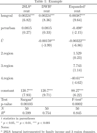
Table 1 provides an empirical example. It uses data provided by the statistical software

Stata for the purpose of illustrating the Sargan test.3 _{For the fifty US states, the data}

comprises rental rates for apartments (rent), next to housing values (hsngval) and the

percentage of the state’s population living in urban areas (pcturban). The housing values

regressor is treated as potentially endogenous in the regression of rents on housing values

and the percentage of urban population at the state level. Median family income and 3

regional dummies - for the state’s central, southern and western areas - are considered as instruments so that there are three over-identifying restrictions. The example shows that

both the Sargan test and the test of the joint significance of ¯Z, the three regional dummies,

reject the null hypothesis of the validity of the over-identifying restrictions.

3

Extension to Nonlinear Models

A nonlinear version of model (1) is given by

y=x(β) +, (19)

where x(·) is a known, differentiable function of β ∈ _Rn1+n2_{. This function is the inverse}

link function in the class of Generalized Linear Models discussed in McCullagh and Nelder

[1983] who also propose an estimation algorithm which amounts to an iterative weighted least squares procedure, a variant of the Newton-Raphson algorithm.

Endogeneity in the nonlinear model amounts to n1 elements of E[∇βx(β)0] being non-zero.4

Davidson and MacKinnon [1990, 1993, 2001] have shown how an “artificial regression”, or Gauss-Newton regression, can be used to test the null hypothesis of exogeneity, i.e.

the consistency of the nonlinear least squares (NLS) estimator ˆβ, under the maintained

hypothesis of a set of valid instruments Z.

2_{The test of the null hypothesis thatδ=0is typically implemented as anF}

m−n1,N−(n2+m+1) test. For

largeN, the squared standard error of the regression ˆσ2

ξ converges in probability toσ2ξ, so that thisF-test

is asymptotically equivalent to aχ2

m−n1 test.

3_{The data can be downloaded from within Stata, usingwebuse hsng2.} 4_{This can be thought of as β}0 _{= (β}0

1, β02), where β1 ∈Rn1 _andβ

2 ∈Rn2_{, andX}

1 =∇β1x(β) satisfying

The NLS estimator solves X ˆ β 0

y−x

ˆ

β

=0, (20)

where X(β) = ∇βx(β) is assumed to have full column rank in a neighborhood about the

true population β.

As an analogue to the residual based exogeneity test in the linear model as implemented in (11),Davidson and MacKinnon [1993] propose the test of the null hypothesis ofτ =0in the regression

y−xβˆ=Xβˆα+ (I−PW)X∗

ˆ

βτ +ζ, (21)

whereX∗ are them−n1-columns ofX that are not annihilated by the orthogonal projector

(I−PW) andW= [X2,Z] is a set ofm+n2instruments.5 The contribution of (I−PW)X∗

ˆ

β

can again be viewed as a set of control functions. This is an artificial or Gauss-Newton

regression because under the null hypothesis one would expect the least squares estimator

of τ to be statistically insignificant. The regressand in this Gauss-Newton regression is

ˆ

=y−x

ˆ

β

.

Now consider the instrumental variable estimator ˜β which satisfies

X ˜ β 0 PW

y−x

˜

β

=0. (22)

The residuals induced by the IV estimator are ˜=y−x

˜

β

. The Sargan test of the validity of over-identifying restrictions is6

TN = ˜0PW˜ (23)

≈ y−x(β)−X(β)

˜

β−β

0

PW

y−x(β)−X(β)

˜

β−β

(24)

=

I−X(β) X ˜ β 0

PWX ˜ β −1 X ˜ β 0 PW ! !0 PW ×

I−X(β)

Xβ˜ 0

PWX

˜

β

−1

Xβ˜ 0 PW ! ! (25)

= 0 PW −PWX(β)

Xβ˜ 0

PWX

˜

β

−1

Xβ˜ 0

PW !

. (26)

Under the null hypothesis, ˜β is consistent forβ, and providedX(·) is continuous,X( ˜β) tends

5_Here,X

2=∇β2x(β), satisfyingE[X

0

2] =0. 6_{In the approximation following the definition ofT}

toX(β) in large samples. Then, under the null hypothesis,TN is asymptotically distributed

χ2

m−n1.

Now consider an expanded Gauss-Newton regression,

ˆ

=Xβˆα+ ¯Zπ+ (I−PW)X∗

ˆ

βτ+ζ, (27)

where ¯Z is an arbitrary subset ofm−n1 columns of Z. Under the null hypothesis, just as in (13), one would expect the least squares estimates ˆπ to be statistically insignificant. Since

PWˆ=PWX

ˆ

β

+ ¯Zπ+PWζ, (28)

it follows that

ˆ

π = π+ Z¯0 I−PWX

ˆ

β

Xβˆ 0

PWX

ˆ

β

−1

Xβˆ 0

PW !

¯

Z

!−1

×Z¯0 I−PWX ˆ β X ˆ β 0

PWX ˆ β −1 X ˆ β 0 PW ! ζ, (29)

a test statistic based on ˆπ satisfies

˜

TN = ˆπ0 Z¯

0

I−PWX

ˆ

β

Xβˆ 0

PWX

ˆ

β

−1

Xβˆ 0 PW ! ¯ Z ! ˆ π (30)

= ζ0 PW −PWX

ˆ

β

Xβˆ 0

PWX

ˆ

β

−1

Xβˆ 0

PW !

ζ. (31)

Under the null hypothesis, ˆβ is consistent for β, and ˜TN is distributed asymptotically

σ2

ζχ2m−n1.

Hence, again, the expanded artificial regression implements the exogeneity and

overiden-tification test is a single regression.

4

Conclusions

This note presents a useful but not widely known framework for jointly implementing

Durbin-Wu-Hausam exogeneity and Sargan-Hansen overidentification tests, as a single artificial regression. It covers linear models and discusses its extension to a class of non-linear models.

Future research might explore how to adapt this methodology to semi-parametric single

approach is already widely employed [Blundell and Powell, 2004, Lee,2007].

References

Richard W. Blundell and James L. Powell. Endogeneity in Semiparametric Binary Response Models. The Review of Economics Studies, 71(3):655–679, 2004.

Russell Davidson and James G. MacKinnon. Specification Tests Based on Artificial

Regressions. Journal of the American Statistical Association, 85(409):220–227, 1990.

Russell Davidson and James G. MacKinnon. Estimation and Inference in Econometrics.

Oxford University Press, 1993.

Russell Davidson and James G. MacKinnon. Artificial Regressions. Queen’s Economics

Department Working Paper No. 1038,, 2001.

James Durbin. Errors in Variables. Review of the International Statistical Institute, 22(1/3):

23–32, 1954.

Lars P. Hansen. Large Sample Properties of Generalized Method of Moments Estimators.

1982.

Jerry A. Hausman. Specification Tests in Econometrics. Econometrica, 46(6):1251–1271,

1978.

Jerry A. Hausman. Handbook of Econometrics, Vol.1, chapter Specification and estimation

of simultaneous equation models, pages 391–448. North Holland, 1983.

Joel Horowitz. Semiparametric and Nonparametric Methods in Econometrics. Springer

Verlag, 2009.

Sokbae Lee. Endogeneity in quantile regression models: A control function approach.Journal

of Econometrics, 141(2):1131–1158, 2007.

P. McCullagh and J.A. Nelder. Generalized Linear Models. Chapman and Hall, 1983.

John D. Sargan. The Estimation of Economic Relationships Using Instrumental Variables.

Econometrica, 26(3):393–415, 1958.

John D. Sargan. Contributions to Econometrics: John Denis Sargan, vol. I, chapter

Testing for misspecification after estimating using instrumental variables, pages 213–235.

De-Min Wu. Alternative Tests of Independence between Stochastic Regressors and

Disturbances. Econometrica, 41(4):733–750, 1973.

A

Tables

Table 1: Example

2SLSa _DWHc _Expandedc

rent rent rent

hsngval 0.00224∗∗∗ 0.00224∗∗∗ 0.00387∗∗∗

(6.82) (8.36) (9.64)

pcturban 0.0815 0.0815 -0.498∗

(0.27) (0.33) (-2.15)

ˆ

U -0.00159∗∗∗ -0.00322∗∗∗

(-3.99) (-6.86)

2.region 1.529

(0.23)

3.region 7.743

(1.14)

4.region -40.61∗∗∗

(-4.62)

constant 120.7∗∗∗ 120.7∗∗∗ 88.27∗∗∗

(7.93) (9.71) (6.22)

Test Sargand _F-teste

p-value 0.00103 0.0002

N 50 50 50

R2 _{0.599 0.754 0.845}

t statistics in parentheses

∗ _{p <0.05,}∗∗ _{p <0.01,}∗∗∗ _{p <0.001}

Notes:

a _{2SLS: hsngval instrumented by family income and 3 region dummies.} b _{Durbin-Wu-Hausman regression.}

c _{Expanded artificial regression, as in equations (12) and (13).} d _{The Sargan test statistic has aχ}2

3distribution. e_{The test statistic has anF}