Fine Grained Work Element Standardization for Project Effort Estimation

http://dx.doi.org/10.4236/jsea.2014.78060

How to cite this paper: Sophatsathit, P. (2014) Fine-Grained Work Element Standardization for Project Effort Estimation. Journal of Software Engineering and Applications, 7, 655-669. http://dx.doi.org/10.4236/jsea.2014.78060

Fine-Grained Work Element Standardization

for Project Effort Estimation

Peraphon Sophatsathit

Department of Mathematics and Computer Science, Faculty of Science, Chulalongkorn University, Bangkok, Thailand

Email: [email protected]

Received 6May 2014; revised 2June 2014; accepted 1July 2014

Copyright © 2014 by author and Scientific Research Publishing Inc.

This work is licensed under the Creative Commons Attribution International License (CC BY).

http://creativecommons.org/licenses/by/4.0/

Abstract

Traditional project effort estimation utilizes development models that span the entire project life cycle and thus culminates estimation errors. This exploratory research is the first attempt to break each project activity down to smaller work elements. There are eight work elements, each of which is being defined and symbolized with visually distinct shape. The purpose is to standard-ize the operations associated with the development process in the form of a visual symbolic flow map. Hence, developers can streamline their work systematically. Project effort estimation can be determined based on these standard work elements that not only help identify essential cost drivers for estimation, but also reduce latency cost to enhance estimation efficiency. Benefits of the proposed work element scheme are project visibility, better control for immediate pay-off and, in long term management, standardization for software process automation.

Keywords

Project Effort Estimation, Work Element, Symbolic Flow Map, Latency Cost, Software Process Automation

1. Introduction

are still subject to validation that involves numerous techniques, which unfortunately are far from maturity. Many researches are underway to arrive at reliably accurate effort estimation techniques, ranging from paramet-ric modeling, knowledge-based modeling, case-based reasoning, statistical inferences, fuzzy logic, neural net-works, and analogies [11] [12]. What follows the underlying method of these models is how well the method performs. This includes errors of measurement, variations in the data sets, and comparative performance statis-tics with other techniques.

This paper will explore a finer grain of project effort estimation based on a well-established measurement paradigm and emerging research endeavors. The study encompasses various viewpoints that propose a break-down of project LC in order to perform finer grained estimate at activity level. Standard operational elements will be defined and put to use. The ultimate goal is to streamline work elements so that the amount of time (which subsequently can be converted to equivalent effort) can be systematically and accurately estimated. Nev-ertheless, whether or not the pros and cons of these novel viewpoints will be applicable to traditional project management, as well as new paradigms of practice such as agile, eXtreme Programming (XP), and Agile Uni-fied Process (AUP), remain to be validated with real project implementation.

This paper is organized as follows. Section 2 recounts some principal building blocks that are applied in many literatures. Section 3 describes traditional project LC estimation, along with Industrial Engineering standard work study, that sets up the proposed fine-grained estimation approach. Section 4 elucidates preliminary com-parative analyses of the proposed breakdown. Suggestions for future direction and prospectus will be discussed in Section 5. Some final thoughts are presented in the Conclusion.

2. Related Work

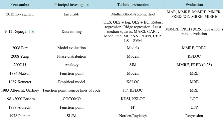
Conventional effort estimation techniques [13] focus on project life cycle data to carry out the project effort and cost involved. Various estimation techniques have been devised to improve estimation accuracy. Table 1 sum-marizes a brief predominant research work and their findings in this area.

A few emerging research endeavors have been attempted to estimate at a finer level using phase-wise project data. Breaking up in phases may uncover activities that were hidden too subjective to measure and average out by LC approach. Different project dimensions can then be taken into account to arrive at a more accurate esti-mation. The empirical findings usually are inapplicable for generic use depending on phase distribution [14]. Various user groups such as IFPUG, ISBSG (International Software Benchmarking Standards Group), are ex-amples of domain specific estimation. Project managers (PMs) must decide what data are to be collected to suit the applicable domain. Jodpimai, Sophatsathit, and Lursinsap [15] explored the relationship of different project dimensions to select only a handful of relevant cost drivers as oppose to standard 16 factors in existing ap-proaches, yet yielding similar outcome. The needs for standardizing its deliverables and development process are key factors to software products. Typical acclaimed standards and working groups are:

 ISO/IEC 14143 [six parts] Information Technology—Software Measurement—Functional Size Measurement  ISO/IEC 19761:2011 Software engineering—COSMIC: A Functional Size Measurement Method

 ISO/IEC 20926:2009 Software and Systems Engineering—Software Measurement—IFPUG Functional Size Measurement Method

657

Table 1. A brief overview of effort estimation research work.

Year/author Principal investigator Techniques/metrics Evaluation

2012 Kocaguneli Ensemble Multimethods/solo method MAR, MMRE, MdMRE, MMER,

PRED (24), MBRE, MIBRE

2012 Dejaeger [16] Data mining

OLS, OLS + log, OLS + BC, Robust regression, Ridge regression, Least

median squares, MARS, CART, Model tree, MLP NN, RBFN, CBR,

LS + SVM

MdMRE, PRED (0.25), Spearman’s rank correlation

2008 Port Model evaluation Models MMRE, PRED

2008 Yang Phase distribution Models KSLOC

2007 Li Analogy SIM MMRE, PRED (0.25)

1994 Matson Function point Models MRE

1987 Kemerer Empirical model KSLOC MRE

1983 Albrecht, Gaffney Function point, source lines of code FP, KSLOC MRE

1981/2000 Boehm COCOMO KDSI, KSLOC LOC

1979 Albrecht Function point FP UFP

1978 Putnam SLIM Norden/Rayleigh Regression

 ISO/IEC 24570:2005 Software Engineering—NESMA Functional Size Measurement Method Version 2.1 —Definitions and Counting Guidelines for the Application of Function Point Analysis

 16326 WG—Information Technology-Software Engineering—Software Project Management Working Group (IEEE)

 ERCIM Working Group Software Evolution

 Project Management Institute (PMI) and Project Management Body of Knowledge (PMBOK®)

While conventional estimation models take the entire LC activities into estimation consideration, finer grained activity breakdown has not been practiced in real software projects. Frederick W. Taylor [17] introduced principles of scientific management in 1911, and Frank B. Gilbreth [18] set up operational work elements that subsequently became work study standard measurement known as Therblig. This study will exploit the use of work element process chart to create fine-grained project activity elements, thereby effort estimation can be de-termined more accurately than current LC practice.

Such a fine-grained breakdown entails phase-wise estimation that in turn permits detailed project visibility. In so doing, this work will attempt to adapt UML style to represent project activity element. Consequently, effort estimation can be managed systematically using standard flow diagrams, activity element set up, and visibly traceable operations.

3. Proposed Fine-Grained Operational Estimation Technique

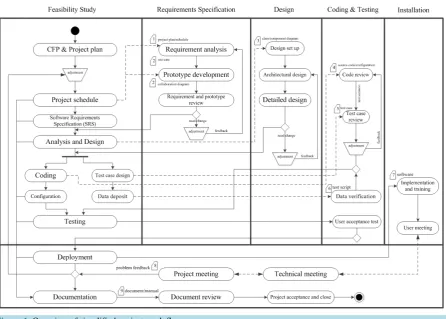
Figure 1. Overview of simplified project work flow.

dotted lines are basically internal information used by developers, while those on solid lines are external infor-mation open to customers. As each activity moves from one phase to the next, efforts are spent on constituent tasks to accomplish the activity. Unfortunately, the work load involved are not straightforwardly and proce-durally described, measured, and collected to determine a reliable estimation. An exploratory research attempt based on well-established Motion and Time Study by Industrial Engineering has been conducted with the hope of setting up work elements in project effort estimation. Figure 2 shows the 18 standard motion elements in Motion and Time Study.

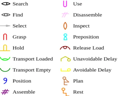
The prime objective of this undertaking is to create visually standard symbols to represent descriptive and subjective constituent smaller tasks of project activity. In so doing, PM and team members can streamline their development process to arrive at a more objectively manageable work flow. Hence, an analogy of Therbligs has been defined in Figure 3 to establish standard work elements involved in each activity. The first element “O” denotes operation to be performed by the team members. Subsequent elements, namely, “D”, “I”, “M”, “T”, “A”, “S”, “P” denote delay, inspection or review, meeting or discussion, movement or transfer, adjustment, storage, and planning or decision, respectively.

Figure 4 illustrates a symbolic flow map of how the activity is procedurally broken down to work elements. The illustration shows a dialog box activity that is broken down to seven smaller tasks proceeding in the follow-ing sequence: O-O-P-M-I-T-T-A-P. This symbolic flow map not only serves as a visual trace of development process work flow, but also a detailed estimation of processing time which can be straightforwardly converted to equivalent effort estimate.

659

Figure 2. Standard 18 motion elements or Therbligs.

Source: Wikipedia (accessed on May 16, 2014).

Figure 3. A novel standard work element definition.

Figure 4. A symbolic flow map of an activity breakdown to work elements.

3.1. Data Collection

The novel approach will utilize conventional waterfall model where each phase is well defined and known by all software developers. As existing standard benchmarking archives such as COCOMO81, NASA93, Desharnais, USP05, MAXWELL1 are available in overall LC figures, this exploratory research will be conducted on a senior elective Software Project Management class to see how this novel scheme can be put to real use.

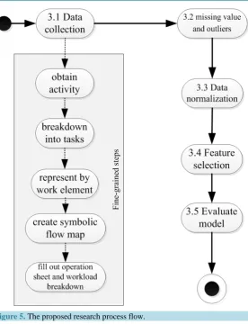
The process began from collecting data of the uppercase phases, i.e., requirements, specification, and design,

Figure 5. The proposed research process flow.

and the lowercase phases, i.e., coding, testing, and implementation. At phase level, functional size measurement [20] such as FP and LOC are employed as high level effort estimation since effort estimation metrics are con-ventionally governed by these two major metrics. Moreover, FP metric can be converted to LOC via backfiring [21]. The information can then be used to estimate overall LC effort. The results so obtained would be used to gauge the accuracy of the proposed fine-grained measurement. Table 2 depicts typical series of activities during the project LC.

An operation data sheet is set up as shown in Figure 6 to record data pertinent to the above symbolic flow map, including idle or overhead that may or may not be prime tasks. Project related data are filled up in the header section, namely, activity, activity ID (primary key), programmer (or group leader), group ID, build, document control number, page, start date, activity duration, project name, and authorized personnel.

661

Figure 6. Operation data sheet.

Table 2. Activities and metrics of project tasks.

Phase activity Input Output Estimation metrics

Software Requirements Specification (SRS) no. of team members Functionality FP

Design no. of requirement/member Functional model FP

Coding Design document Code LOC

Testing no. of rework # errors/module LOC

Implementation no. of transactions from

production code Deliverable Source Instruction LOC

discussion and technical resolution effort with other members of the team except for occasional consultation with test specialist or PM. In this case, allowance may be accounted for as percentage of the test effort which is not considered a prime task. Consequently, the actual activity operation time can be precisely used to determine the equivalent effort estimation, while idle could attribute to latency overhead. The efficiency of operation is di-rectly obtained from utilization factor.

The above operation data are further broken down by team members to depict work load responsibility of each member (shaded area) as shown in Figure 7. Team members are listed on top which contains cross refer-ences to operation data sheet and other related documents. The breakdown permits individual load distribution percentage to be determined accordingly.

A trial collection of work element tallies was taken in order to gauge their distribution based on the governing activity breakdown. These statistics would serve as preliminary effectiveness of fine-grained measures, which in turn could attribute to standardization of activity measurement.

3.2. Missing Value and Outlier

Figure 7. Work load breakdown by team members.

ports. Outlier usually results from freak accidents or exceptional situations where unusually high or low values are recorded. For example, the existence of data singularity in matrix multiplication caused an unusually diffi-cult and extensive test effort to correct, hence the exceptional high effort outlier value.

There are several techniques to handle missing values. One of the most popular and effective techniques is k-nearest neighbor (k-NN) imputation [23]. The technique, as its name implies, uses k data points from the clos- est proximity of the missing value position to interpolate the most likely value. Such an imputation obviously incurs some errors if the actual values are not missing. A viable error estimation is to acquire other projects having the same “feature” value. The use of same feature value from other projects permits cross validation that fills the estimation of missing value to yield more accurate results.

Measuring errors is actually carried out by determining the Euclidean distant between the project having missing values and the ones without. The smaller the average of N measurements, the more accurate the pre-dicted missing values.

Outlier detection is typically handled by examining the kurtosis and skewness of data distribution. Normality test is set up as the null hypothesis using z-score to determine if there exists a significant possibility that null hypothesis is accepted, i.e., normality holds with less than 0.001. This is written as p-value < 0.001. On the con-trary, if the null-hypothesis is rejected, the highest value is treated as the outlier and is discarded. This process is repeated until all outliers are removed.

3.3. Data Normalization

This is a standard technique to linearly scale data of different ranges to the same scale, yet still preserves the re-lationship with the original values. This is done by Equation (1) as follows:

(

)

(

)

max min

ˆ x x ˆ ˆ ˆ

x x x x

x − ×x − +

−

= (1)

where xˆ denotes the reference range, while x denotes individual range.

3.4. Feature Selection

This is the most important activity of project cost estimation. Many existing estimation techniques utilize several cost factors as estimation parameters. For example, the COCOMO model [3] uses 17 cost drivers in the estima-tion process. Jodpimai, Sophatsathit, and Lursinsap [15] found that only a handful of cost drivers were effective factors that could derive as accurate estimation as the comparative models without employing the full-fledge parameter set. Moreover, fewer cost drivers translated into faster computation time. The findings revealed that certain features were vital cost drivers that could yield accurate estimation.

vari-663

ous parameter adjustments during model creation process, whereas the latter is held out for model validation process. The first step is to eliminate independent features that do not contribute or affect project effort estima-tion. The next step is to reduce all redundant features that are less relevant to project effort estimaestima-tion. This is done by means of Pearson’s correlation. Features that result in low value will be less relevant and thus elimi-nated. Finally, only those features that are related to effort estimation in the form of a mathematical function will be retained [15].

There are a number of models that can be used in the feature selection process, ranging from conventional COCOMO, RUP, statistical, and neural network model. The basis for effort estimation must rest on proper use of these selected features in the estimation process, thereby accurate estimation results can be obtained.

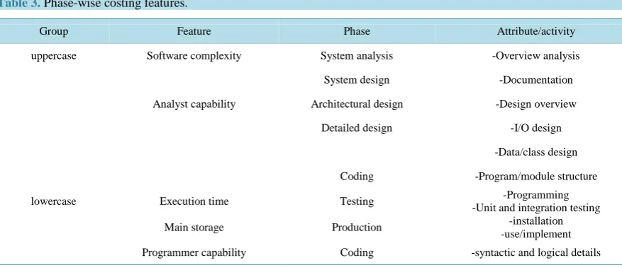
Based on standard 17 cost drivers [3], a phase-wise breakdown and costing features are set up as shown in Table 3 since the project sizes are relatively small, namely, uppercase and lowercase groups. The first group composes of software complexity, analyst capability, while the second group composes of execution time con-straint, main storage concon-straint, and programmer capability. The features will be applied to their corresponding phases.

3.5. Performance Evaluation

There are many performance evaluation methods and their corresponding metrics for effort estimation. Each method has its own applicability to gauge the model accuracy or the relationship between actual and predicted estimation results, given the set of selected features. Table 4summarizes some common methods and metrics for performance evaluation purpose.

Model evaluation is usually carried out by comparing the difference between predicted (estimated) effort y'i

and actual effort yi. Effort is performed on the phase basis using related factors. For example, factors used in

quirements and specification effort estimation involve FP to deal with both functional and non-functional re-quirements. As project requirements become materialized, size estimation via LOC is used instead since it yields more accurate outcome than that of FP. Some metrics are criticized for penalizing over-estimation (such as MRE), while others are just the opposite (such as BRE and MER). Two commonly used metrics are MMRE and PRED (0.25) since they are independent of units of measure and easy to use. However, they are found to give inconsistent results depending on properties of y'i/yi distribution. In which case, MdMRE is used to solve the

outlier problem as MMRE cannot properly handle such inconsistencies. At any rate, this study adopted MMRE and PRED (0.25) accuracy metrics.

A noteworthy shortcoming of this exploratory research endeavor concerns project data. The above procedures have been implemented with industrial projects and extensive public data by the author’s research team, where the resulting outcomes are currently under investigation. The very notion of work element has just been intro-duced after data collection was completed. It was then put to test with classroom environment as it was deemed too novel to be adopted by real projects for the time being. The inherent shortfall of classroom setting was that

Table 3. Phase-wise costing features.

Group Feature Phase Attribute/activity

uppercase Software complexity System analysis -Overview analysis

System design -Documentation

Analyst capability Architectural design -Design overview

Detailed design -I/O design

-Data/class design

Coding -Program/module structure

lowercase Execution time Testing -Programming

-Unit and integration testing

Main storage Production -installation

-use/implement

Pearson’s correlation Relation between two sets of data (estimated

and actual) [27]

(

)

Friedman test Non-parametric hypothesis test as an

alternative to one-way ANOVA [26] 1 1

1 n k

ij

i j

r r

nk = =

=

∑ ∑

Wilcoxon matched pairs signed-rank test

Non-parametric as an alternative to parametric

paired simple t-test [28] x2,i−x1,isgn

(

)

Kruskal-Wallis ANOVA test Non-parametric as alternative one-way

ANOVA > 3 samples [29] ( )

( )

(

)

N r r

K r r = = = = − −

∑

∑ ∑

project size was too small to warrant any reliable practice or significance.

4. Preliminary Analyses

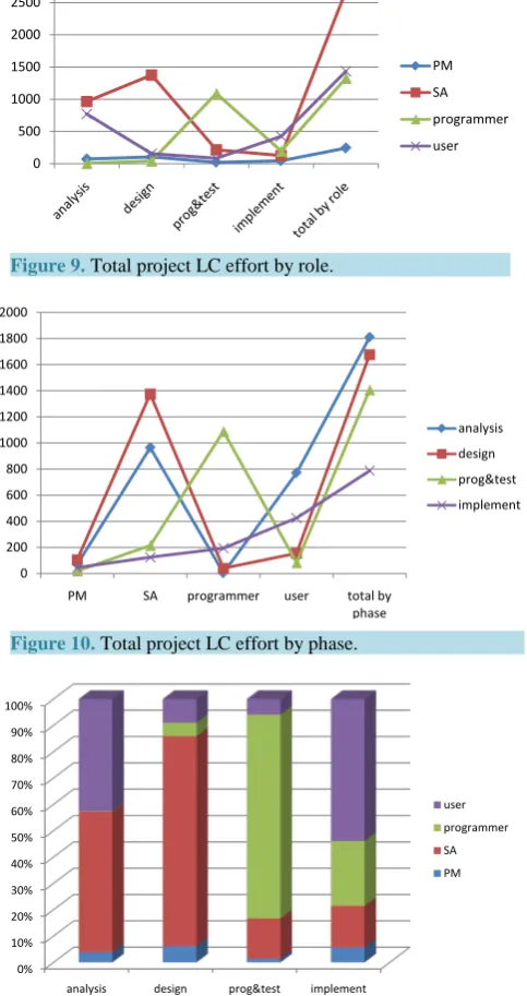
This exploratory research sets out to compare the proposed measurement with that of traditional LC. Due to the small number of students enrolled in the class, the samples were not a good representative of any conclusive in-ferences. Anyhow, the above procedures were followed to ensure that pertinent data were properly collected. Each team consisted of a project manager (PM), a system analyst (SA), a programmer, and a user. Students were asked to estimate phase effort that they would expend. These estimates would be used as the target values to be compared with the fine-grained figures from operation data sheet. They also collected actual LC efforts on class assignment by role and by development phases.Figure 8 depicts work element histogram of individual’s load distribution of the dialog box task based on the breakdown in Figure 7. Figure 9 and Figure 10 show the total project LC effort (y-axis) expended by role and by phase, respectively.

Table 5summarizes individual’s load distribution based on operation data sheet. In analysis phase, the pro-grammer played very little role in the assignment. Thus, his contribution in this phase was virtually non-existent (0.3%), while SA did most of the work in the first two phases and gradually reduced his role afterwards. The programmer made up for the loss in programming and testing, and the user participated heavily during the in-ception (analysis) phase and the closing (implementation) phase. Figure 11 shows the resulting plot.

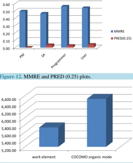
Table 6 and Figure 12 show the value of MMRE and PRED (0.25) and corresponding plot of the class. The predictions from work elements of all parties fluctuated somewhat to the actual value as MMRE was moderate and PRED was not significant enough to yield any close predictions. The deviation was resulted from excessive allowances that were quite difficult to administer. This was a pioneer attempt to undertake something of this na-ture in Software Engineering which, on the contrary, has been well established with supporting standards in In-dustrial Engineering.

Table 7 and Figure 13 show the result comparison of total project effort obtained from COCOMO estimation in organic mode with the actual work element count by the proposed method. The reason being organic mode was that students were familiar and experienced with project development process. Work element breakdown was additional clerical tasks that they had to do as part of project documentation. The effort discrepancies were likely precipitated from fine-grained measurements having fewer latency cost.

665

Figure 8.Individual’s work element distribution of the dialog box task.

Figure 9. Total project LC effort by role.

Figure 10. Total project LC effort by phase.

Figure 11.Work load distribution plot.

0 500 1000 1500 2000 2500 3000

PM SA programmer user

0 200 400 600 800 1000 1200 1400 1600 1800 2000

PM SA programmer user total by phase

analysis design prog&test implement

0% 10% 20% 30% 40% 50% 60% 70% 80% 90% 100%

analysis design prog&test implement

Figure 13.Actual total work element effort VS COCOMO organic mode estimation plot.

Table 5. Work load distribution from operation data sheet.

Analysis Design Prog & test Implement Total by role

PM 71 106 20 45 242

SA 964 1375 215 124 2678

Programmer 4 88 1091 194 1377

User 771 155 83 425 1434

Total by phase 1810 1724 1409 788

Table 6. MMRE and PRED (0.25) values.

MMRE PRED (0.25)

PM 0.49 0.00

SA 0.46 0.04

Programmer 0.56 0.03

User 0.54 0.04

Overall 0.52 0.03

Table 7.Actual total work element effort VS COCOMO estimation.

Measurement Effort

Work elememt 5732.00

COCOMO Organic mode 6515.44

5,200.00 5,400.00 5,600.00 5,800.00 6,000.00 6,200.00 6,400.00 6,600.00

667

member was well aware of his own assignment and the course of action with other team members. The posted symbolic flow map of each activity (which could be posted in the so called “project war room”) proved to be an extremely valuable tracking tool during a “sit down” meeting to discuss the course of action, effort spent, and possibly (which rarely happened) activity reassignment. This attributed to finer grained analysis that portrayed a more visible activity tracking, not to mention more accurate measurements which in turn lessened the estimation errors. From a practical standpoint, the risk of over/under estimation is reduced, thereby improving project esti-mation and bidding opportunity.

5. Findings and Future Direction

This survey sets out to explore fine-grained project cost estimation, aiming at more accurate result than using traditional LC approach. Admittedly, the novelty of such an undertaking does not offer much provision for overall project management. All experimental data were improvised from classroom assignments. As mentioned earlier, performance could not be measured accurately due to the small sample size and unfamiliarity with work element notion. Fortunately, students were special group of people that possessed exceptional abilities, i.e., fast learning, flexibility, and adaptability. These attributes bring new work disciplines and culture to modern project management know-how. That is why this study embarks on a new realm of fine-grained measurement to cope with such a revolutionary transformation. The findings unveil some noteworthy results that have potential bene-fits to software project management.

 modern software products are short-live which cannot fit into traditional LC analysis. The proposed fine- grained approach could open a new realm of exploiting development process standard to foster some forms of subjective project task measurements.

 fine-grained analysis can be adapted to cope with more scrutinized investigation provided that appropriate metrics and analysis techniques are applied.

Benefits from this exploratory estimation proposal can be summarized as follows:

1) Operational work element is an inherent, not accidental characteristic of project management [30]. The na-ture of software development process irrespective of the underlying model lends itself to collecting data which are readily available. What has not been done is the breakdown of activity structure. In addition, the difficulty of data collection process is seen as disruptive and infeasible as many tasks are operationally in-tertwined. This makes it hard to succinctly separate.

2) Modern development paradigms are seen to be unfitted to LC estimation. As the term “phase” has been in-grained in software engineering since the inception of waterfall model and has become a stigma of software project management. A closer look into this investigation reveals that if the term is viewed as a milestone of partial work products that can be accurately measured by a well-established standard, the term can be gener-alized to cover all paradigms of software development. For example, some “standard” work elements in the dialog box task can be reused elsewhere by other tasks in the project, thus reducing the time and effort to set up and measure similar tasks. As work elements become standardized, development process can be stream-lined and automatically generated to attain software automation.

3) Various available tools, techniques, and metrics can be tailored to fit work element operation without having to reinvent the wheel. The available software body of knowledge (SWEBOK) can be straightforwardly adapted and exploited by software PM.

4) Training to work with systematic operating procedures and assessments in this fine-grained measurement is required. Proper planning must be carried out to set up the necessary programs for all personnel involved. 5) The advent of smart phone technology offers unlimited avenues for software research and development. As

such, newer development paradigms and management techniques are called for. Undoubtedly, the success of such an undertaking can be tailored to support project estimation and streamline the development process.

6. Conclusions

This exploratory research proposes a novel work element standardization to streamline software development process. The ultimate goal is to reach software automation, wherein tasks can be automated succinctly. A num-ber of benefits can be drawn from such an elaborative attempt. They are:

that makes up for high quality software products. Future software process automation can be realized as well.

References

[1] Putnam, L. (1978) A General Empirical Solution to the Macro Software Sizing and Estimating Problem. IEEE Trans-actions on Software Engineering, SE-4, 345-361. http://dx.doi.org/10.1109/TSE.1978.231521

[2] Boehm, B. (1981) Software Engineering Economics. Prentice Hall PTR, Upper Saddle River.

[3] Boehm, B., Abts, C., Brown, A., Chulani, S., Clark, B., Horowitz, E., Madachy, R., Reifer, D. and Steece, B. (2000) Software Cost Estimation with COCOMO II. Prentice Hall PTR, Upper Saddle River.

[4] Walston, C.E. and Felix, C.P. (1977) A Method of Programming Measurement and Estimation. IBM Systems Journal,

16, 54-73. http://dx.doi.org/10.1147/sj.161.0054

[5] Bailey, J.W. and Basili, V.R. (1981) A Meta-Model for Software Development Resource Expenditures. Proceedings of the 5th International Conference on Software Engineering, 107-116.

[6] Albrecht, A.J. and Gaffney Jr., J.E. (1983) Software Function, Source Lines of Code, and Development Effort Predic-tion. IEEE Transactions on Software Engineering, SE-9, 639-648. http://dx.doi.org/10.1109/TSE.1983.235271

[7] Kemerer, C.F. (1987) An Empirical Validation of Software Cost Estimation Models. IEEE Transactions on Software Engineering, 30, 416-429.

[8] Matson, J.E., Barrett, B.E. and Mellichamp, J.M. (1994) Software Development Cost Estimation Using Function Points. IEEE Transactions on Software Engineering, 20, 275-287. http://dx.doi.org/10.1109/32.277575

[9] Albrecht, A. (1979) Measuring Application Development Productivity. I. B. M. Press, New York, 83-92. [10] Karner, G. (1993) Resource Estimation for Objectory Projects. Objective Systems SF AB.

[11] Shepperd, M. and Schofield, C. (1997) Estimating Software Project Effort Using Analogies. IEEE Transactions on Software Engineering, 23, 736-743. http://dx.doi.org/10.1109/32.637387

[12] Li, J.Z., Ruhe, G., Al-Emran, A. and Richter, M.M. (2007) A Flexible Method for Software Effort Estimation by Analogy. Empirical Software Engineering, 12, 65-106. http://dx.doi.org/10.1007/s10664-006-7552-4

[13] Nasir, M. (2006) A Survey of Software Estimation Techniques and Project Planning Practices. Proceedings of the sev-enth ACIS International Conference on Software Engineering, Artificial Intelligence, Networking, and Paral-lel/Distributed Computing (SNPD’06), Las Vegas, 19-20 June 2006, 305-310.

[14] Yang, Y., He, M., Li, M., Wang, Q. and Boehm, B. (2008) Phase Distribution of Software Development Effort. Pro-ceedings of the Second ACM-IEEE International Symposium on Empirical Software Engineering and Measurement

(ESEM’08), Kaiserslautern, 9-10 October 2008, 61-69.

[15] Jodpimai, P., Sophatsathit, P. and Lursinsap, C. (2010) Estimating Software Effort with Minimum Features using Neural Functional Approximation. Proceedings 2010 International Conference on Computational Science and Its Ap-plications (ICCSA), Fukuoka, 23-26 March 2010, 266-273. http://dx.doi.org/10.1109/ICCSA.2010.63

[16] Dejaeger, K., Verbeke, W., Martens, D. and Baesens, B. (2012) Data Mining Techniques for Software Effort Estima-tion: A Comparative Study. IEEE Transactions on Software Engineering, 38, 375-397.

http://dx.doi.org/10.1109/TSE.2011.55

[17] Taylor, F.W. (1911) The Principles of Scientific Management. Harper & Brothers, New York and London, LCCN11010339, OCLC233134.

669

[19] Kocaguneli, E., Menzies, T. and Keung, J.W. (2012) On the Value of Ensemble Effort Estimation. IEEE Transactions on Software Engineering, 38, 1403-1416. http://dx.doi.org/10.1109/TSE.2011.111

[20] Gencel, C. and Demirors, O. (2008) Functional Size Measurement Revisited. ACM Transactions on Software Engi-neering and Methodology, 17, 15:1-15:36.

[21] Jones, C. (1995) Backfiring: Converting Lines of Code to Function Points. Computer, 28, 87-88.

http://dx.doi.org/10.1109/2.471193

[22] Tsunoda, M., Kakimoto, T., Monden, A. and Matsumoto, K.-I. (2011) An Empirical Evaluation of Outlier Deletion Methods for Analogy-Based Cost Estimation. Proceedings of the 7th International Conference on Predictive Models in Software Engineering, Banff, 20-21 September 2011, 17:1-17:10.

[23] Keller, J.M., Gray, M.R. and Givens, J.A. (1985) A Fuzzy K-nearest Neighbor Algorithm. IEEE Transactions on Sys-tems, Man and Cybernetics, SMC-15, 580-585. http://dx.doi.org/10.1109/TSMC.1985.6313426

[24] Kitchenham, B., Pickard, L., MacDonell, S. and Shepperd, M. (2001) What Accuracy Statistics Really Measure [Soft-ware Estimation]. Proceedings IEE—Software, 148, 81-85.

[25] Foss, T., Stensrud, E., Kitchenham, B. and Myrtveit, I. (2003) A Simulation Study of the Model Evaluation Criterion MMRE. IEEE Transactions on Software Engineering, 29, 985-995.

http://dx.doi.org/10.1109/TSE.2003.1245300

[26] Friedman, M. (1937) The Use of Ranks to Avoid the Assumption of Normality Implicit in the Analysis of Variance.

American Statistical Association, 32, 675-701. http://dx.doi.org/10.1080/01621459.1937.10503522

[27] Abran, A. and Robillard, P. (1996) Function Points Analysis: An Empirical Study of Its Measurement Processes. IEEE Transactions on Software Engineering, 22, 895-910. http://dx.doi.org/10.1109/32.553638

[28] Redei, G.P. (2008) Encyclopedia of Genetics, Genomics, Proteomics and Informatics. Springer, Heidelberg.

[29] de Vries, D. and Chandon, Y. (2007) On the False-Positive Rate of Statistical Equipment Comparisons Based on the Kruskal-Wallis HStatistic.IEEE Transactions on Semiconductor Manufacturing, 20, 286-292.

http://dx.doi.org/10.1109/TSM.2007.901398