New Edge Detection Enhancement Method based on Cooperation between Edge Algorithms

(1)

New Edge Detection Enhancement Method based on

Cooperation between Edge Algorithms

Ashraf A. Nijim

Faculty of Engineering Al-Azhar University,

Cairo, Egypt.

Muhammad T. Abo

Kresha

Ph.D

,

Faculty of Science Al-Azhar University,

Cairo, Egypt.

Reda Abo Alez

Prof., Faculty of Engineering Al-Azhar University,

Cairo, Egypt.

ABSTRACT

Edge detection algorithms are important tools in image processing applications for carrying out much information and being relatively easy to produce. Sobel; Canny; and logarithmic algorithms [1] are among several edge detection algorithms used frequently nowadays. The evalution of such edge detection algorithms is an old problem. Authors [1][3] tend to use visual evaluation that limits the comparison between different edge images. In this paper, we present a new edge enhancement method and five different measures that can be used to statistically evaluate edge detection algorithms. The new edge enhancement method is based on cooperation between different edge detection algorithms. The new edge preserves the advantages of each edge image. Experimental results using two edge detection algorithms proved the efficiency of this method.

General Terms

New Edge Enhancement Method; Pattern Recognition; Edge Detection Algorithms; Image Entropy; and Image Moments.

Keywords

Edge detection; Canny edge detector; Sobel edge detector; logarithmic edge detector; MSE; PSNR; PCC; Shannon Entropy; Hu-moments.

1. INTRODUCTION

Edge detection algorithms differ in their performance for different types of images. The most well- known edge detection algorithms are: Canny [1][2]; Sobel [1]; and logarithmic [1]. The performance of edge detection algorithms was evaluated in two ways: visual and numerical. Visual [1][3] means of testing the performance of edge detection algorithms has been adopted for many years because of the lack of standard measuring techniques whereas, numerical evaluation methods tend to reflect the visual difference between the object and its evaluated edge. Authors [4] and [5] used two numerical methods for evaluating the difference between two images. The Mean Square Error (MSE); the Peak Signal-to-Noise Ratio (PSNR); and Pearson’s Correlation Coefficient (PCC) were used to indicate how much two images are numerically different. The entropy [8][9] and moments [10][11] of images were also used in many recognition algorithms and image processing algorithms [10][11][12].

This paper is organized as follows: Section 2 deals with edge detection algorithms. Section 3 deals with edge evaluation. Section 4 presents the new edge enhancement method. Section 5 deals with the edge evaluation results. Section 6 deals with the new edge enhancement results. Section 7 deals with the discussion part of the results, and Section 8 deals with the conclusions of this study.

2. EDGE DETECTION ALGOITHMS

Authors [13][14] provided different definitions for the edge of a given image. The definition of an edge for a given object that best satisfies our study purpose is: An edge is a set of connected pixels of width one that lies on the boundary of two regions. Inner-edge is the boundary of some region that lies inside the edge of that region. And, the outer-edge is the set of pixels that lies exactly outside the boundary of a region.

In the following section, three different edge detection algorithms will be described.

2.1 Sobel Edge Detector

The Sobel edge detector [1] is a simple non-linear edge detection technique. It uses two 3X3 filters to find the differencing scheme in an image.

𝐿𝑒𝑡 𝑎 ∈ ℝ𝑋_{𝑏𝑒 𝑡𝑕𝑒 𝑠𝑜𝑢𝑟𝑐𝑒 𝑖𝑚𝑎𝑔𝑒, 𝑎𝑛𝑑}

𝐿𝑒𝑡 𝑚 ∈ ℝ𝑋_{𝑏𝑒 𝑡𝑕𝑒 𝑔𝑟𝑎𝑑𝑖𝑒𝑛𝑡 𝑚𝑎𝑔𝑛𝑖𝑡𝑢𝑑𝑒 𝑖𝑚𝑎𝑔𝑒}

Then, Sobel edge magnitude image 𝑚 is defined as follows:- 𝑚 𝑖, 𝑗 ∶= 𝑎⨁𝑠 2_{+ 𝑎⨁𝑡}2_,

where the templates 𝑠 and 𝑡 are defined as follows:-

𝑠 =−1 −2 −1 0 0 0 1 2 1

, 𝑎𝑛𝑑 𝑡 =

−1 0 1 −2 0 2 −1 0 1 The gradient direction 𝑑 could be found using the following formula:-

𝑑 = 𝑎𝑟𝑐𝑡𝑎𝑛2 (𝑎 ⊕ 𝑠) 𝑚>0 , (𝑎 ⊕ 𝑡) 𝑚>0

2.2 Canny Edge Detector

Canny edge detection [1][2] is a multi-stage image processing algorithm. The squared gradient magnitude is computed first. Edges are then identified as the local maxima of this magnitude if its value exceeds a predefined threshold. Canny’s algorithm was designed to achieve three optimization constrains:-

i. Good detection by maximizing the signal to noise ratio. ii. Good localization to accurately mark edges.

iii. Respond only once to a single edge in a 1-D signal.

2.3 Logarithmic (Wallis) Edge Detector

The logarithmic edge detection [1] uses the difference between the log value of a given pixel and its neighbors to find the edge pixels. If the value exceeds a predefined threshold then this pixel is an edge pixel.

𝐿𝑒𝑡 𝑎 ∈ ℝ𝑋_{𝑏𝑒 𝑡𝑕𝑒 𝑠𝑜𝑢𝑟𝑠𝑒 𝑖𝑚𝑎𝑔𝑒, 𝑎𝑛𝑑}

(2)

the edge image 𝑏 ∈ ℝ𝑋is given by, 𝑏 𝑖, 𝑗 = log𝑏 𝑎 𝑖, 𝑗

−1

4 log𝑏 𝑎0

+ log𝑏 𝑎1 + log𝑏 𝑎2 + log𝑏 𝑎3

The previous equation can be extended to include more than 4-neighbors for wider comparison.

3. EDGE EVALUATION

Following are five image techniques used to statistically evaluate images:

3.1 MSE

The Mean Square Error (𝑀𝑆𝐸) [4] for two images 𝐼 and 𝐾 is defined as follow:-

𝑀𝑆𝐸 = _𝑚∗𝑛1 𝑛−1[𝐼 𝑖, 𝑗 − 𝐾(𝑖, 𝑗)]2 𝑗 =0

𝑚 −1

𝑖=0 ,

Where 𝑚 ∗ 𝑛 is the size of the image.

3.2 PSNR

The Peak Signal-to-Noise Ratio (𝑃𝑆𝑁𝑅) [5] is defined as follows:-

𝑃𝑆𝑁𝑅 = 10 log

₁₀

(

𝑀𝐴𝑋_𝑀𝑆𝐸2

)

,

where MAX is the maximum pixel value the image can have.

3.3 Pearson’s Correlation Coefficient (PCC)

The Pearson’s Correlation Coefficient (PCC)[17][18] is defined as follows:-

Where,

𝑥𝑖 is the intensity of the 𝑖𝑡𝑕 pixel in image1,

𝑦𝑖 is the intensity of the 𝑖𝑡𝑕 pixel in image2, 𝑥𝑚 is the mean intensity of image1, and

𝑦𝑚 is the mean intensity of image2.

The correlation coefficient returns a value between 1 and -1. A value of 1 indicates that the two images are identical, a 0 that the images are completely uncorrelated, and -1 indicates that the images are completely anti-correlated for example if the image is a negative of the other.

3.4 Central Moments

The central moments 𝜇𝑝𝑞 [11] of a function 𝑓(𝑥, 𝑦) are defined

as follows:-

𝜇𝑝𝑞 = 𝑥 − 𝑥 𝑝 𝑦 − 𝑦 𝑞 𝑏2

𝑏1

𝑎2

𝑎1

Shannon entropy [8][9]is defined as a measure of the average information content associated with a random outcome. Shannon entropy 𝐻 𝑋 for discrete random variable 𝑋, with possible states 𝑥1, 𝑥2, … , 𝑥𝑛 is defined as follows:-

𝐻 𝑋 = 𝑝 𝑥𝑖 log2 _{𝑝 𝑥}1 𝑖 = − 𝑛

𝑖=1

𝑝 𝑥𝑖 log2𝑝(𝑥𝑖) 𝑛

𝑖=1

,

where, 𝑝 𝑥𝑖 = 𝑃𝑟(𝑋 = 𝑥𝑖) is the probability of the 𝑖𝑡𝑕

outcome of 𝑋.

4. NEW ENHANCEMENT METHOD

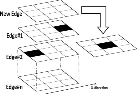
The proposed new edge enhancement method is based on different edge detection algorithms selection. Two or more of well-known edge detection algorithms coordinate to find a new edge. The new edge reserves the benefits of each of those edge algorithms. The edge enhancement method is composed of three steps: The first step is referred as the x-direction edge selection. The pseudo code for this step is as follows:-

For each place (pixel) in the new edge image:

 Check if the pixels in the right side x-direction of the different n-edge images have one or more edge pixel, if True, then;

 Check if the pixels in the left side x-direction of the different n-edge images have one or more edge pixel, if True, then;

[image:2.595.317.541.503.655.2]

 Set that pixel to black-edge pixel (see Figure 2). Fig 1: The pseudo code for the x-direction edge selection

(3)

The second step is referred as the y-direction edge selection. The pseudo code for this step is as follows:-

For each white (non-edge) place in the new edge image:

 Check if the pixels in the right side y-direction of the different n-edge images have one or more edge pixel, if True then;

 Check if the pixels in the left side y-direction of the n-edge images have one or more n-edge pixel, if True, then;

[image:3.595.346.498.70.226.2]

 Set that white pixel to black-edge pixel (see Figure 4). Fig 3: The pseudo code for the y-direction edge selection

Fig 4: Second step, y-direction edge selection

The third and final step is a post edge enhancement step. In this step the new edge image is investigated to remove any artifacts during the two selection steps and to make sure that the new edge is of one pixel width.

5. EDGE EVALUATION RESULTS

In this section, we will investigate the relationship between the original image and its edge images. Three edge detection algorithms –Sobel; Canny; and logarithmic- are used on two groups of image. The first group is composed of binary images with different geometric shapes (see Figure 5). The second group of images is a database of colored retina images [6][7]. A sample of this database is shown in Figure 6. Evaluation was done using the five methods presented in section 3. A Sample of the results from the first group of images is presented in Table 1. (Geom1) binary image was evaluated with its three edge images.

[image:3.595.60.286.230.387.2]

Fig 5: Geometric shapes test image (Geom1)

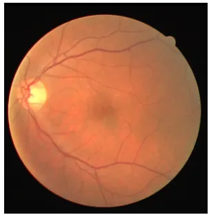
Fig 6: Retina test image, 21_training.tif (Ret2)

[image:3.595.312.540.297.462.2]

The comparison results for both images are shown in Table 1 and Table 2.

Table 1. Test image (Figure 5) evaluation results

Test\Image Original Canny Sobel Log.

MSE --- 9384 9425 9637

PSNR --- 69.990 69.971 69.874 PCC --- 0.0800 0.0630 -0.0142 Shannon

Entropy

0.6849 0.1507 0.1505 0.1589 Hu Moments

(𝜙1)

0.2183 0.1675 0.1675 0.1675

Hu Moments (𝜙₂)

3.5778 3.6720 3.6720 3.6719

Hu Moments (𝜙₃)

1.6784 3.9394 x10-4

3.7803 x10-4

4.4733 x10-4 Hu Moments

(𝜙4)

12.0395 7.1347 x10-4

7.1164 x10-4

[image:3.595.312.540.524.689.2]

13.2040 x10-4 Sample evalution results for the second group of images are presented in Table 2. Ret2 gray scaled image was evaluated with its three edge images.

Table 2. Retina image (Figure 6) evaluation results

MSE --- 18950 17594 18390

PSNR --- 60.539 60.861 60.669 PCC --- -.1490 .0190 -.1103 Shannon

Entropy

6.4890 1.7072 .3214 1.4177 Hu Moments

(𝜙₁)

0.1950 0.1801 0.1675 0.1740

Hu Moments (𝜙2)

3.6224 3.6374 3.6613 3.6486

0.5944 1.4127 x10-2

1.7038 x10-4

(𝜙₄)

1.1236 10.660 1 x10-2

3.9537 x10-4

(4)

[image:4.595.310.541.75.478.2]

degrees CW (see Table 3 b) and (see Table 4 b); and 70 degrees CW (see Table 3 c) and (see Table 4 c).

Table 3. Test image (Figure 1) comparison results (a) Rotation 20 CW

MSE --- 9422 9407 9594

PSNR --- 69.972 69.979 69.894 PCC --- 0.0699 0.0609 0.0021 Shannon

Entropy

0.8310 0.2227 0.1736 0.1948 Hu Moments

(𝜙₁)

0.2183 0.1679 0.1675 0.1677

Hu Moments (𝜙2)

3.5800 3.6712 3.6720 3.6717

1.6777 9.1944 x10-4 3.5178 x10-4 4.9706 x10-4 Hu Moments

(𝜙4)

17.5424 21.396 2 x10-4

8.1267 x10-4

14.523 3 x10-4

(b) Rotation 45 CW

MSE --- 9411 9413 9582

PSNR --- 69.977 69.976 69.899 PCC --- 0.0740 0.0585 0.0050 Shannon

Entropy

0.8377 0.2373 0.1849 0.2081 Hu Moments

(𝜙1)

0.2183 0.1679 0.1674 0.1676

3.5795 3.6712 3.6721 3.6717

1.6757 10.160 7 x10-4

3.6387 x10-4

(𝜙4)

19.0190 16.178 8 x10-4

8.6183 x10-4

11.536 5 x10-4

(c) Rotation 70 CW

MSE --- 9418 9410 9589

PSNR --- 69.974 69.978 69.896 PCC --- 0.0696 0.0582 1.2165 x10-4 Shannon

Entropy

0.8330 0.2273 0.1796 0.1944 Hu Moments

(𝜙₁)

0.2183 0.1679 0.1674 0.1676

Hu Moments (𝜙2)

3.5760 3.6711 3.6720 3.6716

1.6794 8.3108 x10-4 4.0501 x10-4 5.9954 x10-4 Hu Moments

(𝜙4)

17.0861 18.289 4 x10-4

8.3968 x10-4

14.101 8 x10-4

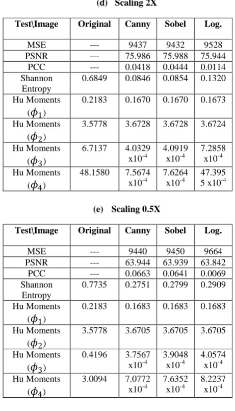
(d) Scaling 2X

MSE --- 9437 9432 9528

PSNR --- 75.986 75.988 75.944 PCC --- 0.0418 0.0444 0.0114 Shannon

Entropy

0.6849 0.0846 0.0854 0.1320 Hu Moments

(𝜙1)

0.2183 0.1670 0.1670 0.1673

3.5778 3.6728 3.6728 3.6724

6.7137 4.0329 x10-4 4.0919 x10-4 7.2858 x10-4 Hu Moments

(𝜙4)

48.1580 7.5674 x10-4

7.6264 x10-4

47.395 5 x10-4

(e) Scaling 0.5X

MSE --- 9440 9450 9664

PSNR --- 63.944 63.939 63.842 PCC --- 0.0663 0.0641 0.0069 Shannon

Entropy

0.7735 0.2751 0.2799 0.2909 Hu Moments

(𝜙₁)

0.2183 0.1683 0.1683 0.1683

3.5778 3.6705 3.6705 3.6705

Hu Moments (𝜙3)

0.4196 3.7567 x10-4 3.9048 x10-4 4.0574 x10-4 Hu Moments

(𝜙₄)

3.0094 7.0772 x10-4

7.6352 x10-4

8.2237 x10-4

Table 4. Retina image (Figure 2) comparison results (a) Rotation 20 CW

MSE --- 20793 19487 20329

PSNR --- 60.136 60.417 60.234 PCC --- -.1450 -.0011 -.1177 Shannon

Entropy

6.5123 1.7612 0.3770 1.4350 Hu Moments

(𝜙1)

0.1934 0.1803 0.1677 0.1747

3.6153 3.6361 3.6607 3.6475

0.5413 2.0446 x10-2 4.4937 x10-4 2.6411 x10-2 Hu Moments

(𝜙₄)

1.2305 15.850 5 x10-2

43.934 9 x10-4

8.9174 x10-2

(b) Rotation 45 CW

MSE --- 21640 20226 21088

[image:4.595.310.542.499.768.2]

(5)

x10-4 Shannon

Entropy

6.4254 1.7697 0.3680 1.4245 Hu Moments

(𝜙₁)

0.1929 0.1805 0.1677 0.1747

3.6086 3.6357 3.6610 3.6479

0.5872 1.0556 x10-2

2.9235 2.2604 x10-2 Hu Moments

(𝜙₄)

2.2153 0.2552 42.047 5 x10-4

0.1320

(c) Rotation 70 CW

MSE --- 20785 19497 20383

PSNR --- 60.137 60.415 60.222

PCC --- -.1407 3.8123

x10-4

-.1231 Shannon

Entropy

6.5236 1.7892 0.3728 1.4675 Hu Moments

(𝜙₁)

0.1934 0.1804 0.1677 0.1749

3.6102 3.6359 3.6610 3.6470

Hu Moments (𝜙3)

0.6429 68.254 5 x10-4

3.1777 1.4964 x10-2 Hu Moments

(𝜙₄)

3.0342 0.3283 33.279 1 x10-4

0.1652

(d) Scaling 2X

MSE --- 18730 17594 18438

PSNR --- 66.616 66.882 66.678 PCC --- -.1417 -.0052 -.1187 Shannon

Entropy

6.4805 1.5674 0.2318 1.6274 Hu Moments

(𝜙₁)

0.1950 0.1779 0.1673 0.1794

3.6224 3.6411 3.6616 3.6378

2.3777 4.0783 x10-2

10.751 1 x10-4

(𝜙₄)

4.4936 0.2179 30.357 5 x10-4

0.1826

(e) Scaling 0.5X

MSE --- 19250 17586 18207

PSNR --- 54.442 54.835 54.684 PCC --- -0.1663 0.0443 -0.0817 Shannon

Entropy

6.4927 1.8969 0.4716 1.1199 Hu Moments

(𝜙₁)

0.1950 0.1826 0.1678 0.1715

Hu Moments 3.6217 3.6307 3.6599 3.6529

(𝜙2) Hu Moments

(𝜙₃)

0.1495 1.0039 x10-2

1.6742 x10-5

(𝜙₄)

0.2798 3.3730 x10-2

5.2696 x10-5

0.5355 x10-2

6. NEW EDGE ENHANCMENT RESULTS

The new method was tested using three images. The true edges of those images were extracted manually. The first test image is the binary image (Geom1) which has five different geometric shapes. The size of this image is 1200x1200 pixels (see Figure 5).

[image:5.595.337.500.259.417.2]

The two other test images are texture mosaic images from the USC-SIPI web site database[15][16] (see Figure 7 and Figure 8).

Fig 7: Texture Mosaic Image, texmos2.s512.tiff (Texm1)

Fig 8: Texture Mosaic Image, texmos3.s512.tiff (Texm2)

[image:5.595.337.499.436.592.2]

(6)

[image:6.595.48.289.88.257.2]

Table 5. Canny, Sobel and the new edge comparison results

Image name

Test/ Edge Alg.

Canny vs. True Edge

Sobel vs. True Edge

NewEdge vs. True

Edge

Geom1

MSE 2288x10-6 2930 x10-6 2261 x10-6 PSNR 87.9886 86.9141 88.0390

Texm1

MSE 4082 x10-5 3711 x10-5 4077 x10-5 PSNR 68.0757 68.4901 68.0818

Texm2

MSE 1512 x10-5 1611 x10-5 1508 x10-5 PSNR 72.3894 72.1135 72.3993

The comparison results showed an improvement in the new edge image compared to both Canny and Sobel edge images. The MSE was reduced, showing that the two edge images – the new edge image and the true edge image – are getting closer to each other. The Sobel edge results for the texture mosaic image (Texm1) is found to be better than both Canny and the New Edge images. This result is expected because Sobel edge detection algorithm proved to give accurate detection for edges parallel to the x and y directions. In this special case, (Texm1) has all of its edges parallel to either the x or the y directions (see Figure 6).

Figure 9 shows parts from the first test image (Geom1). The resulting new edge image has improved. Corners and oblique lines are closer to the original image than both edge detection algorithms - Canny and Sobel. Even more, the new method improved the Sobel edge by adding the missing pixels from the edge.

(a) Original (b) Canny Edge (c) New Edge

(a) Original (b) Sobel Edge (c) New Edge

Fig 9: Edge enhancement, (a) Parts from (Geom1) (Figure 5); (b) Edge detection results using Canny and Sobel; (c)

New edge enhancement image.

7. DISCUSION

The MSE values between the original image and its edge images represent the inner non-edge pixels of the objects in the image, and the edge identification errors. Those errors include misplaced edges and noise added by the edge identification algorithm. The value of MSE is greater than zero sincea zero MSE value is only found when comparing two identical images. MSE between the edge and its original image does not change with rotation or scaling for simple geometric shapes (see Figure 5). This value slightly changes with complex images (see Figure 6). From our observation this change did not exceed 4%.

The PSNR represents a ratio of change for two images to the maximum possible value of an image. The same discussion can be said about the PSNR. However, the change of PSNR values after rotation and scaling didn’t exceed 1% for both simple and complex images. This makes the PSNR value more favorable. The value of the PCC proved that the edge images and the original image are not correlated. The PCC values are close to zero for both images. Most of the values are positive for the first image (Geom1) but negative for the second image (Ret2). The edge image doesn’t provide that much information as the original image provides. This explains the great change in entropy value between the original image and the different edge images.

The first and the second Hu-moments (𝜙1 𝑎𝑛𝑑 𝜙2) of the

images is observed to have the same value for the different edge images (see Table 1, and Table3) for simple geometric shapes. For complex images those values start to set apart. But, the second Hu-moments (𝜙2) was observed to have identical values with the original image moments after scaling (see Table 4 d and e). The second Hu-moments for the complex retina image (Ret2) and its three edge images were observed to have common values.

The new edge enhancement results showed that the new proposed method improved edge detection. The cooperation between two or more edge detection algorithms using relatively simple techniques provided better edge detection. Using only two edge images, better angles and oblique lines detection were achieved. The MSE and PSNR values proved this improvement for the two sample images. Both values have been computed using manually generated true edge images. Those true edge images may not represent the true edge for some algorithms because of inconsistency in defining edges.

8. CONCLUSION

Cooperation between two or more edge detection techniques proved to give better edge detection. The results after using the new method with two edge detection algorithms showed a significant improvement in edge detection. The angles and oblique lines of Canny and Sobel edge images were properly detected. Statistical results using manually generated true edge images showed that the new edge image and the true image were closer than both edge images.

MSE and PSNR between edge images and the original image were observed to have identical values under rotation and scaling. Difference in those values represents the change in edge detection for two algorithms. The higher the MSE value, the more complex the image is. Shannon entropy [8][9] value for the edge images is lower than the entropy of the original image. This is due to the fact that the edge image does not carry that much information the original image does.

[image:6.595.54.274.455.597.2]

(7)

9. REFERENCES

[1] Ritter, G. X., and Wilson J. N. 2001. Handbook of Computer Vision Algorithms in Image Algebra. Second Edition. CRC Press.

[2] Ali, M., and Clausi, D. 2001. Using The Canny Edge Detector for Feature Extraction and Enhancement of Remote Sensing Images. IEEE Geoscience and Remote Sensing Symposium. 2298-2300.

[3] Shrivakshan, G.T., and Chandrasekar, C., 2012. A Comparison of various Edge Detection Techniques used in Image Processing. IJCSI International Journal of Computer Science Issues, Vol. 9, Issue 5, No 1. 269-276.

[4] Tan, H. L., Li, Z., Tan, Y. H., Rahardja, S., and Yeo C. 2013. A perceptually Relevant MSE-Based Image Quality Metric. IEEE Transactions on Image Processing, Vol. 22, No. 11. 4447-4459.

[5] Huynh-Thu, Q., and Ghanbari, M. 2008. Scope of validity of PSNR in image/video quality assessment. Electronic Letters, Vol. 44, Issue 13. 800-801.

[6] Staal, J.J., Abramoff, M.D., Niemeijer, M., Viergever, M.A., and van Ginneken, B. 2004. Ridge based vessel segmentation in color images of the retina. IEEE Transactions on Medical Imaging, vol. 23. 501-509. [7] Niemeijer, M., Staal, J.J., van Ginneken, B., Loog, M., and

Abramoff, M.D. 2004. Comparative study of retinal vessel segmentation methods on a new publicly available database. SPIE Medical Imaging, Vol. 5370. 648-656. [8] Shannon, C. E. 1948. A Mathematical Theory of

Communication. Bell System Technical Journal, 27 (3). 379–423.

[9] Shannon, C. E., and Weaver, W. 1949. The Mathematical Theory of Communication. University of Illinois Press.

[10]Hu, M. K. 1961. Pattern recognition by moment invariants, Proc. IRE49. 1428.

[11]Hu, M. K. 1962. Visual problem recognition by moment invariant. IRE Trans. Inform. Theory. Vol. IT-8. 179-187. [12]Rizon, M., Yazid, H., Saad, P., Shakaff, A. Y., Saad, A.,

Mamat, M. R., Yaacob, S., Desa, H., and Karthigayan, M. 2006. Object Detection using Geometric Invariant Moment. American Journal of Applied Science 2 (6). 1876-1878.

[13]El-Sayed, M. 2011. A New Algorithm Based Entropy Threshold for Edge Detection in Images. IJCSI International Journal of Computer Science Issues. Vol. 8, Issue 5, No 1. 71-78.

[14]Vidya, P., Veni, S., and Narayanankutty K. A. 2009. Performance Analysis of Edge Detection Methods on Hexagonal Sampling Grid. International Journal of Electronic Engineering Research. Vol. 1, No. 4. 313-328. [15]Signal and Image Processing Institute. The USC Texture

Mosaic Images. USC University of Southern California. http:// sipi.usc.edu.

[16]Laws, K. I. 1980. Textured Image Segmentation. PhD thesis, University of Southern California. USCIPI. Report 940.

[17]Neto, A. M., Rittner, L., Leite, N., Zampieri, D. E., Lotufo, R., and Mendeleck, A. 2007. Pearson’s Correlation Coefficient for Discarding Redundant Information in Real Time Autonomous Navigation System. IEEE Multi-conference on Systems and Control, Cingapura.