PV boost converter conditioning using neural network

PV BOOST CONVERTER CONDITIONING USING NEURAL NETWORK

AIZAT BIN ABD AZIZ

A project report submitted in partial fulfillment of the requirement for the award of the

Degree of Master of Electrical Engineering

Faculty of Electrical and Electronic Engineering Universiti Tun Hussein Onn Malaysia

ABSTRACT

ABSTRAK

CONTENTS

TITLE i

DECLARATION ii

DEDICATION iii

ACKNOWLEDGEMENT iv

ABSTRACT v

ABSTRAK vi

CONTENTS vii

LIST OF TABLES x

LIST OF FIGURES xi

LIST OF SYMBOLS AND ABBREVIATIONS xiv

LIST OF APPENDICES xv

CHAPTER 1 INTRODUCTION 1

1.1 Project Background 1

1.2 Problem Statement 2

1.3 Project Objective 2

1.4 Project Scope 3

CHAPTER 2 LITERATURE REVIEW 4

2.1 Literature survey on existing model of neural network DC-DC converter

4

2.2 Solar Energy 5

2.3 Photovoltaic Technology 5

2.4 Base Transceiver Station 7

2.5 Boost Converter 9

2.5.1 Analysis for the Switch Closed 10 2.5.2 Analysis for the Switch Open 11 2.5.3 Steady State Operation 12 2.5.4 Boost Converter Modes of Operation 13 2.6 Artificial Neural Network (ANN) 14

2.7 PID Controller 17

CHAPTER 3 METHODOLOGY 19

3.1 Project Design 19

3.2 Modelling of Boost Converter 20 3.2.1 Average State-Space Representation for

DC-DC Boost Converter

20

3.3 Proposed neural network controller (NNC) architecture

23

3.4 Training the Neural Network Controller 25 3.5 Modelling of Solar PV Module 26

3.5.1 Solar Cell Model 26

2.5.2 Photovoltaic Module 28

CHAPTER 4 RESULT AND ANALYSIS 32

4.1 Boost Converter Using Open Loop System 32 4.1.1 Pulse Width Modulation (PWM) 33 4.1.2 Open Loop Boost Converter Subsystem 34

4.1.2.1 Boost converter output voltage result for variant setting of duty cycle

4.2 Solar Model Simulation Result 36 4.3 Closed Loop PV Boost Converter Using PID

Controller

37

4.3.1 Simulation result for PV boost controller using PID

39

4.4 Closed Loop PV Boost Converter Using Neural Network Controller

40

4.4.1 Simulation Result For PV Boost Controller Using Neural Network

43

4.5 Performance Comparison Between PV Boost Converter Using Neural Network And PID.

44

4.5.1 Simulation result comparison for Neural Network and PID controller response

45

4.5.1.1 Simulation result for sun irradiance at 1200 W/m2

46

4.5.1.2 Simulation result for sun irradiance at 1000 W/m2

47

4.5.1.3 Simulation result for sun irradiance at 800 W/m2

48

4.5.1.4 Simulation result for sun irradiance at 600 W/m2

49

4.5.2 Summary of performance for Neural Network and PID controller

50

4.5.3 Simulation result for daily actual sun irradiance data in Subang, Selangor.

51

CHAPTER 5 CONCLUSION AND FUTURE

RECOMMENDATION

54

5.1 Conclusion 54

5.2 Future Recommendation 55

REFERENCES 56

LIST OF TABLES

3.1 Parameters of the boost converter 22

3.2 Solar cell parameters 28

4.1 Boost converter components value 33 4.2 Deviation of voltage resulted from open loop circuit Boost

Converter

34

4.3 Value for KP, KI and KD 38

4.4 Comparison of boost output voltage with the reference voltage for PID controller

40

4.5 Output voltage for variant number of neurons used in hidden layer

41

4.6 Comparison of boost output voltage with the reference voltage for neural network controller

44

4.7 Time duration of sun irradiance 45 4.8 Comparison of boost output voltage with the reference voltage

for Neural Network and PID controller.

50

4.9 Actual irradiance raw data taken from Subang Metereological Station, Selangor, Malaysia

51 4.10 Output voltage produced for each of the actual irradiance data

taken in Subang, Selangor, Malaysia.

LIST OF FIGURES

2.1 Base Transceiver Station (BTS) 7 2.2 Base Transceiver Station tower 7 2.3 Scheme of conventional BTS (P. A. Dahono et al,. 2009). 8 2.4 Base Transceiver Station using renewable energy (P. A. Dahono

et al,. 2009).

9

2.5 Boost converter 9

2.6 Boost equivalent circuit for the switch closed 10 2.7 Waveforms for inductor voltage and current during switch closed 10 2.8 Boost equivalent circuit for the switch opened 11 2.9 Waveforms for inductor voltage and current during switch

opened

11

2.10 Inductor current waveform in CCM and DCM modes 14 2.11 Schematic of a Biological Neuron 14

2.12 Multilayer perceptron 16

2.13 PID controller structure 18

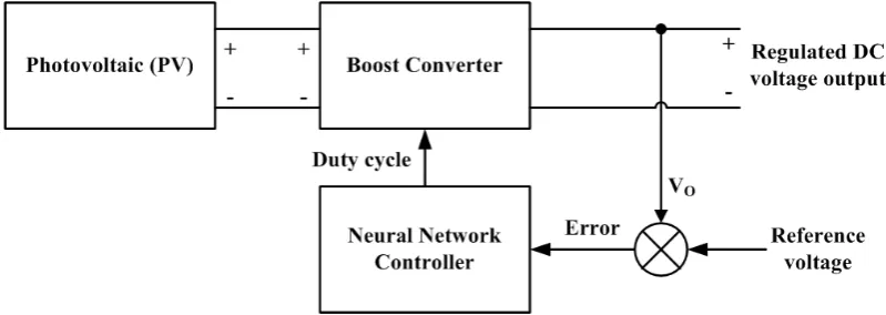
3.1 Block diagram of the proposed PV boost system control by neural network controller

19

3.2 DC – DC Boost converter 20

3.3 Simulink diagram of state space averaged model of the boost converter

22

3.10 Solar cell simulink block 26 3.11 The equivalent circuit for solar block model 27 3.12 Solar photovoltaic module consist of 72 solar cells 28 3.13 The parallel connection of 36 solar cells inside a solar

photovoltaic module

29

3.14 The parallel connection of 18 solar cells inside 36 solar cells block

29

3.15 The parallel connection of 6 solar cells inside 18 solar cells block 29 3.16 The series connection of 6 solar cells 30 3.17 The complete circuit connection of solar photovoltaic module 31 4.1 Open-loop modelling of Boost DC-DC converters 32

4.2 PWM design 33

4.3 Duty cycle waveform 33

4.4 Subsystem for open loop boost converter 34 4.5 Output voltage for duty cycle, D = 0.2 35 4.6 Output voltage for duty cycle, D = 0.4 35 4.7 Output voltage for duty cycle, D = 0.6 35 4.8 Output voltage for duty cycle, D = 0.8 36

4.9 Solar model 36

4.10 Effect of irradiance to solar output voltage 37 4.11 PV boost system using PID controller 38 4.12 Modelling design of PID controller 38 4.13 Boost converter and solar voltage using PID Controller 39 4.14 Simulation of Irradiance reading from the sun 39 4.15 PV boost system using Neural Network controller 40 4.16 Two layer feed-forward neural network 41

4.17 Mean squared error 42

4.18 Error histogram 42

4.19 Function fit between output and target 43 4.20 Boost converter and solar voltage using Neural Network

Controller

43

4.22 Comparison of boost output voltage response when using Neural Network or PID Controller

45

4.23 Comparison of boost output voltage response when using Neural Network or PID Controller for sun irradiance at 1200 W/cm2

46

4.24 Settling time for Neural Network and PID controller for sun irradiance at 1200 W/cm2

46

4.25 Comparison of boost output voltage response when using Neural Network or PID Controller for sun irradiance at 1000 W/cm2

47

4.26 Settling time for Neural Network and PID controller for sun irradiance at 1000 W/cm2

47

4.27 Comparison of boost output voltage response when using Neural Network or PID Controller for sun irradiance at 800 W/cm2

48

4.28 Settling time for Neural Network and PID controller for sun irradiance at 800 W/cm2

48

4.29 Comparison of boost output voltage response when using Neural Network or PID Controller for sun irradiance at 600 W/cm2

49

4.30 Settling time for Neural Network and PID controller for sun irradiance at 600 W/cm2

49

4.31 Performance of Neural Network and PID controller in terms of settling time

50

4.32 Daily irradiance data in Subang, Selangor, Malaysia 52 4.33 Neural Network response towards different value of actual

irradiance data in Subang, Selangor, Malaysia.

52

LIST OF SYMBOLS AND ABBREVIATIONS

PV - Photovoltaic DC - Direct Current PWM - Pulse Width Modulation

PID - Proportional integral derivative Control ANN - Artificial Neural Network

BTS - Base Transceiver Station GSM - Global System for Mobile CDMA - Code Division Multiple Access

WAN - Wide Area Network AC - Alternate Current CCM - Continuous Current Mode DCM - Discontinuous Current Mode

VL - Inductor Voltage VS - Supply Voltage

iL - Inductor Current Δ - Small Constant Value T - Time

D - Duty Cycle Vo - Output Voltage

LIST OF APPENDICES

APPENDIX TITLE PAGE

CHAPTER 1

INTRODUCTION

1.1 Project background

Renewable energy has become a higher priority for both research and industry communities due to natural gas and pollution have increased, and considerable attempts to find sources of energy efficiency have been made extensively. Photovoltaic systems (PV), which convert sunlight into electricity, has been regarded as one of the potential alternative because there is no fuel costs, low maintenance costs, low operating costs and no sound. PV systems are classified into three types, namely, grid-connected systems, stand-alone and hybrid. All types require an electronic interface between the solar panel system for either direct current or alternating load [1].

Traditional design techniques are based on Proportional-Integral-Derivative (PID) controllers in which parameters can be adjusted for appropriate settling-time, overshoot and specific output values according to Mohamed Elshaer [2]. However, the PID controller is not sufficient for non-linear systems. Hence, an Artificial Neural Network (ANN) has become proficient solution for non linear system controls [3], with the capability of learning problems and predicts the next solution.

In this project, the output voltage control system for boost converter integrated with PV model is studied with the purpose of controlling a specific output voltage under input voltage variation caused by changes in irradiation of the solar cells. The ANN control technique is used to regulate the output voltage. The application of this system is to supply a constant dc 48V to Base Transceiver Station (BTS) that used in telecommunication system according to P. A. Dahono [4].

1.2 Problem statement

Photovoltaic (PV) system, which converts sunlight into electricity is not always received an optimum sun irradiation everyday. The sudden changes in irradiation will cause the output voltage of the PV system varies. Therefore the stand-alone PV system without an electronics interface system between the output of the PV system and the load is not suitable to be used to supply power to an application that required a constant dc supply to be operated such as Base Transceiver Station (BTS) telecommunication equipment that required a 48V dc input supply.

1.3 Project objective

The objectives of this project are:

i. To develop a simulation of PV boost converter using Neural Network controller to control a specific output voltage under input voltage variation caused by changes in irradiation of the solar cells.

1.4 Project scope

The scopes of this project is to simulate the proposed method of stabilize the output voltage of the Boost converter by using Neural Network Controller (NNC) with MATLAB Simulink software. Neural network controller will be design based on a two-layer feed-forward network with sigmoid hidden neurons and linear output neurons and train by using Levenberg-Marquardt back-propagation algorithm.

1.5 Thesis overview

This thesis is organized into five chapters. The structure and description of the thesis can be described as follows.

Chapter 1 describes about project background, problem statement, project objectives and project scope. Chapter 2 covers the literature review of previous case study based on neural network controller background and development. Besides, general information about renewable energy, Base Transceiver Station, Boost Converter and theoretical revision on neural network control system also described in this chapter. Chapter 3 presents the methodology used to design open loop Boost Converter and neural network controller.

CHAPTER 2

LITERATURE REVIEW

2.1 Literature survey on existing model of neural network DC-DC converter

Since neural network controller can mimic human behaviour, many researchers applied neural network controller to control voltage output. A thorough literature overview was done on the usage of neural network controller as applied in DC-DC Boost Converter.

N. Jiteurtragool, C. Wannaboom and W. San-Um [1], proposed a power control system in DC-DC Boost converter integrated with photovoltaic arrays using optimized back propagation artificial neural network by using MATLAB simulink software. The simulation result shows the neural network controller possesses fast settling time of 6.4ms with low voltage ripples of approximately 0.625%.

Ivan Petrović, Ante Magzan, Nedjeljko Perić and Jadranko Matuško [6], proposed a neural control of boost converter input current by using MATLAB simulink software. The simulation result shows that the neural network controller provides much better responses of the input current than PI controller: 15 times shorter settling time, 2 times better ripples attenuation and responses without overshoots in opposite to 35% overshoots. Besides, it is much easier to adjust neural network controller then the PI controller.

B. S. Dhivya, V. Krishnan and Dr. R. Ramaprabha [7], proposed a Neural Network Controller for Boost Converter by using MATLAB simulink software. The simulation result shows that the ANN based controller proves to have a fast response in tracking the desired output voltage and is also effective ill decreasing overshoot, oscillations and settling time.

2.2 Solar Energy

Solar energy is energy that is extracted from the radiation released from the sun in the form of heat and electricity. This energy is essential to all life on earth. It is a renewable source of clean, economical, and less pollution than other sources of energy [8]. Therefore, solar energy is rapidly gaining notoriety as an important means of expanding renewable energy resources. Therefore, it is important that people understand the technology of engineering associated with this area.

2.3 Photovoltaic Technology

into electricity. Improving solar module efficiencies while holding down the cost per cell is an important goal of the PV industry.

Cristalline silicon (monocrystalline or polycristalline) and Thin Film are the two main photovoltaic technologies.

 Crystalline silicon

Made from thin slices cut from a single crystal of silicon (monocrystalline) or from a block of silicon crystals polycrystalline), with an efficiency ranging between 11% and 20%. This technology represents about 85% of the market today

 Thin Film

Made by depositing extremely thin layers of photosensitive materials onto a low-cost backing such as glass, stainless steel or plastic. Lower production costs counterbalance this technology’s lower efficiency rates (from 5% to 13% average)

 Other cell types

2.4 Base Transceiver Station

A base transceiver station (BTS) as shown in Figure 2.1 below is a piece of equipment that facilitates wireless communication between user equipment (UE) and a network which required dc 48V input power supply [4]. The location of the BTS is inside a BTS tower as per Figure 2.2. UEs are device like mobile phones, computers with wireless internet connectivity and others. The network can be that of any of the wireless communication technologies like GSM, CDMA, wireless local loop, WAN, WiFi, WiMAX and others.

Figure 2.1: Base Transceiver Station (BTS)

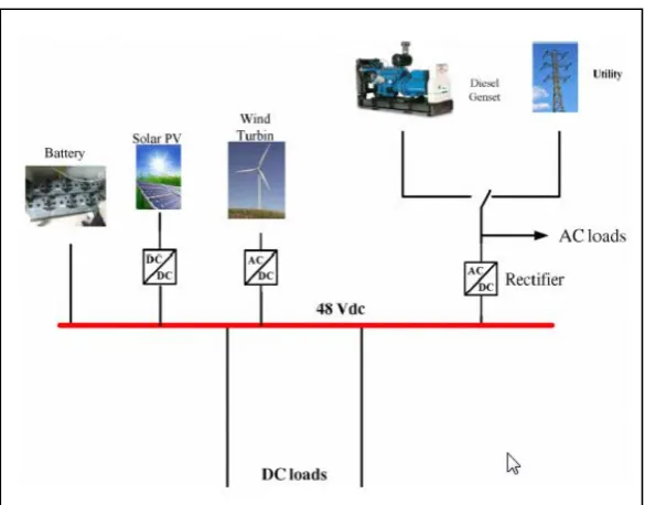
BTS conventional power system scheme is shown in Fig. 2.3. BTS is usually power-driven by utility lines. A diesel generator is typically used as back-up. Air conditioning and lighting systems are powered from the AC bus. By using rectifiers, AC power is converted into 48V dc power. Batteries and telecommunication equipment connected directly to 48V dc bus. These batteries are typically designed to provide at least 6 hours of back-up time. In rural areas, however, diesel generator is usually the main source. For small BTSs, around 2000 liters of diesel fuel needed each month. In rural areas or small islands, the main problem is how to deliver the fuel. Just in several years, the fuel cost may exceed the price of the BTS itself [4].

Figure 2.3: Scheme of conventional BTS [4]

Figure 2.4: Base Transceiver Station using renewable energy (P. A. Dahono et al,. 2009).

2.5 Boost converter

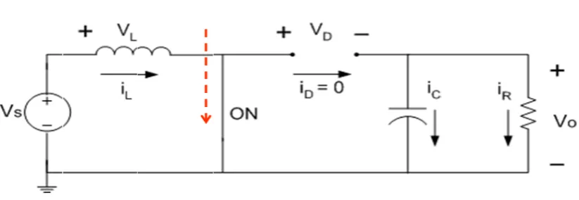
The boost converter is shown in Figure 2.5. This is a switching converter that operates by periodically opening and closing an electronic switch. It is called a boost converter because the output voltage is larger than the input [9].

Figure 2.5: Boost converter

2.5.1 An

Figure 2.6 closed.

When the around the

The rate o switch is c

Figure

nalysis for t

6 below sho

Figure

e switch is e path conta

of change of closed, as sh

e 2.7: Wave

V

the Switch

ows the equi

2.6: Boost

closed, the aining the so

f current is hown in Fig

eforms for i

d L V =

V_{L s} 

Closed

ivalent circu

equivalent c

e diode is ource, induc a constant, gure 2.7. inductor vol or d d dt di_L

uit of boost

circuit for th

reverse bia ctor, and clo

so the curre

ltage and cu

L V = dt

di_{L s}

t converter d

he switch c

ased. Kirch osed switch

ent increase

urrent during

during the s

losed

hhoff’s volt h is

es linearly w

g switch clo

switch is

tage law

(2.1)

while the

The chang Solving fo 2.5.2 An Figure 2.8 opened. Figure 2.9 the switch Figure

ge in inducto

or ΔiL for th

nalysis for t

8 below sho

Figure

9 below sho h is opened. 

e 2.9: Wave

or current is

he switch cl

the Switch

ows the equi

2.8: Boost e

ows the ind

eforms for in Δd

Δi = dt

di_{L L}

 

s computed losed, Open ivalent circu equivalent c ductor voltag nductor volt D Δ T Δi = dt _ON L L _



uit of boost

circuit for th

ge and indu

tage and cu

L V = DT

Δi_{L s}

DT

   

t converter d

he switch op

uctor curren

urrent during

during the s

pened

nt waveform

g switch ope

(2.2)

(2.3)

switch is

m during

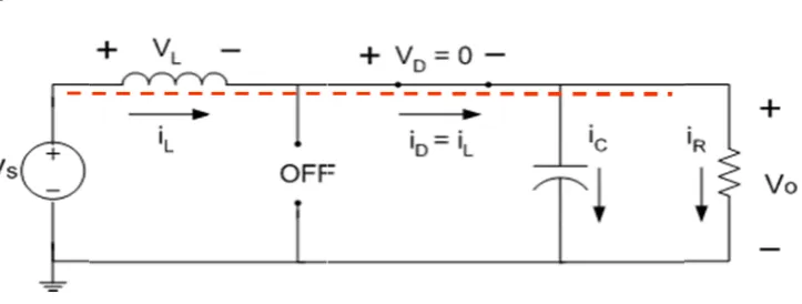
When the switch is opened, the inductor current cannot change instantaneously, so the diode becomes forward-biased to provide a path for inductor current. Assuming that the output voltage Vo is a constant, the voltage across the inductor is

(2.4)

The rate of change of inductor current is a constant, so the current must change linearly while the switch is open. The change in inductor current while the switch is opened is

(2.5)

Solving for ΔiL for the switch opened,

(2.6)

2.5.3 Steady state operation

For steady-state operation, the net change in inductor current must be zero. Using Equation (2.3) and (2.6),

Solving for Vo

(2.7) dt di L V V = V L o s

L  

L V V = dt

di_{L s}  _o

 L V V = D)T ( Δi T Δi = Δdt Δi = dt

di _{L s o}

OFF L L L    1

 

L V V =

Δi s o

opened

L  

The average current in the inductor is determined by recognizing that the average power supplied by the source must be the same as the average power absorbed by the load resistor. Output power is

(2.8)

and input power is Vs Is = Vs IL. Equating input and output powers and using Equation (2.7),

(2.9)

By solving for average inductor current and making various substitutions, IL can be expressed as

(2.10)

Maximum and minimum inductor currents are determined by using the average value and the change in current from Equation (2.3).

(2.11)

(2.12)

2.5.4 Boost Converter modes of operation

The DC-DC converters can have two distinct modes of operation: Continuous conduction mode (CCM) and discontinuous conduction mode (DCM). In practice, a converter may operate in both modes, which have significantly different characteristics. However, this project only considers the DC-DC converters operated in CCM. CCM used for efficient power conversion and Discontinuous Conduction Mode DCM for low power or stand-by operation [10].

o o o

o V I

R V =

P 2 

R D) ( V = R D V = I V s s L s 2 2 2 1 1         R D) ( V = I s

L _1 2

Figure 2.10 below shows the inductor current condition for CCM and DCM modes.

Figure 2.10: Inductor current waveform in CCM and DCM modes

2.6 Artificial Neural Network (ANN)

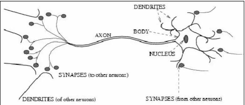
Artifical neural network are computational networks which attempt to simulate the network of biological central nervous system. The human brain is made of millions of individual processing elements that are highly interconnected. A schematic of single biological neurons is shown in Figure 2.11.

Figure 2.11: Schematic of a Biological Neuron

by the diffusion of ions. These synapses connect to the cell inputs, or dendrites and the single output of the neuron appears at the axon [5].

Artificial neural networks are made up of individual models of the biological neuron connected together to form a network. These neuron models are simplified versions of the actions of a real neuron. In simulating a biological neuron network, artificial neural networks allow using simple computational operations to solve complex, mathematical ill-defined and non-linear problems.

Another important feature of artificial neural networks is its learning capability. The learning mechanism is often achieved by appropriate adjustments of the weights in the synapses of the artificial neuron models. Training is done by non-linear mapping or pattern recognition. If an input set of data corresponds to a definitive signal pattern, the network can be trained to give correspondingly a desired pattern at the output. This capability to learn is due to the distributed intelligence contributed by the weights which can be done either online or offline. A properly trained neural network is able to generalize to new inputs by providing sensible outputs when presented with a set of input data that is has not been exposed to.

The simplest artificial neural network model is based on the McCulloch-Pitts neurons defined by Warren S. McCulloch and Walter Pitts in 1943. This neuron was static and did not include changing input weights. It dealt with variable inputs multiplied with fixed synaptic weight, with the product being summed. If this sum exceeded the neurons threshold, the neuron turned on or stayed on. If the sum was below the threshold of an inhibitory pulse was received, the neuron turned off or stayed off. The output of the neuron, y(i), is represented by:

(2.13)

Where wi is the weight value, xi is the input and n represent the number of inputs. In 1958, Frank Rosenblatt put together a learning machine, the perceptron by modifying the McCulloch-Pitts and Hebb models. This merged the concepts of synapse changes as a function of activity as well as the effects of combining multiple inputs to a single neuron. The perceptron is the simplest form of neural network consisting of a single neuron with adjustable synaptic weights and bias. This model is limited to performing pattern classification with only two linearly separable classes. The perceptron forms the basis of an adaline (adaptive linear neuron)



i wixi

proposed by B. Widrow in 1960. This is a single neuron model involving weight training according to the least square error algorithm, defined by the following equation:

(2.14)

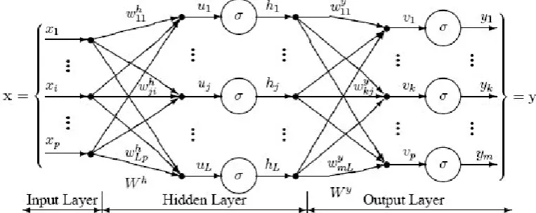
Where W is the desired weight, is the current weight, e(i) is the error term calculated by taking the difference between the desired and actual output, x(i) is the input to the neuron and η is the learning rate. The above mentioned can be generalized under a specific class known as the single layer perceptron (SLP). Another popular artificial neural network architecture is the multiple layer perceptron (MLP). This network consists of an input layer, a number of hidden layers and output layer as shown in Figure 2.12.

Figure 2.12: Multilayer perceptron

Theoutput of each node is connected to the inputs of all the nodes in the subsequent layer. Data flows through the network in one direction from input to output. The network is trained in a supervised fashion involving both network inputs and target outputs.

Back-propagation (BP) is a supervised learning technique used for training artificial neural networks. It was first described by Paul Werbos in 1974 and further developed by David E. Rumelhart, Geoffrey E. Hinton and Ronald J. Williams in 1986. As the algorithm’s name implies, the errors (and therefore the learning) propagate backwards from the output nodes to the inner nodes. So technically, BP is used to calculate the gradient of the error of the network with respect to the network’s modifiable weights. This gradient is almost always used in a simple



 

i

i x i e W

W  ( ) ()

stochastic gradient descent algorithm to find weight that minimizes the error. It is important to note that BP networks are necessarily multilayer (usually with one input, one hidden and one output layer). In order for the hidden layer to serve any useful function, multilayer networks must have non-linear activation functions for the multiple layers, whereas a multilayer network using only linear activation functions is equivalent to a single layer, linear network. Non-linear activation functions that are commonly used include the logistic function, the softmax function and the Gaussian functions.

2.7 PID Controller

Most of the control techniques in industrial applications are embedded with the Proportional-Integral-Derivative (PID) controller. PID control is one of the oldest techniques. It uses one of its families of controllers including P, PD, PI and PID controllers. There are two reasons why nowadays it is still the majority and important in industrial applications. First, its popularity stems from the fact that the control engineer essentially only has to determine the best setting for proportional, integral and derivative control action needed to achieve a desired closed-loop performance that obtained from the well-known Ziegler-Nichols tuning procedure.

A proportional integral derivation controller (PID Controller) is a generic control loop feedback mechanism widely used in industrial control system. A PID is most commonly used feedback controller. Over 90% of the controllers in operation today are PID controllers (or at least some form of PID controller like a P or PI controller). This approach is often viewed as simple, reliable, and easy to understand.

Typical steps for designing a PID controller are;

i. Determine what characteristics of the system need to be improved. ii. Use KP to decrease the rise time.

iii. Use KD to reduce the overshoot and settling time. iv. Use KI to eliminate the steady-state error.

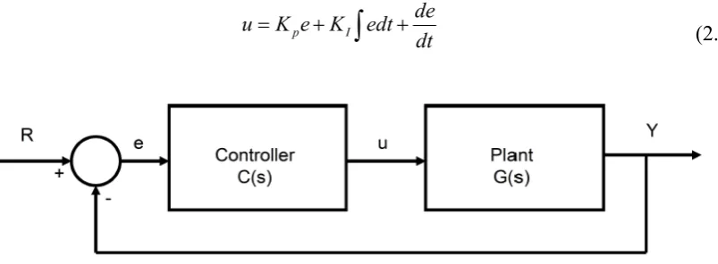
Equation below shows the mathematical equation of designing a PID controller based on the Figure 2.13.

(2.15)

Figure 2.13: PID controller structure

The variable e denotes the tracking error, which is sent to the PID controller. The control signal u from the controller to the plant is equal to the proportional gain (KP) times the magnitude of the error plus the integral gain (KI) times the integral of the error plus the derivative gain (KD) times the derivative of the error.



 

dt de edt K e K

CHAPTER 3

METHODOLOGY

3.1 Project design

Figure 3.1 below shows a project block diagram. Photovoltaic (PV) will supply input voltage to the boost converter depending on the value of sun irradiation. The neural network controller function is to adjust the necessary duty cycle to ensure that the boost converter will produce output voltage that will equal to the reference voltage.

3.2 Modelling of boost converter

3.2.1 Average State-Space representation for dc-dc boost converter

The ideal dynamics of the boost converter are derived by the state space averaging method. The boost converter of Figure 3.2 below with a switching period of T and a duty cycle of D is given. The converter will be operating in a continuous conduction mode (CCM) and the state space equations when the main switch is ON are shown by equation below [11]. 

1 ( )

, 0 , : 1 _{( )}

L

in

o o

di

V

dt L _{t dT Q ON}

dv v

dt C R

 _  _{ }   _{ }         (3.1)

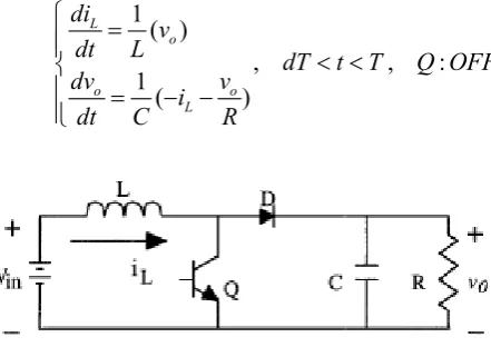
State space equations when the main switch in OFF are shown by equation below.

1_{( )}

, , : 1 ( ) L o o o L di v

dt L _{dT t T Q OFF}

dv v

i

dt C R

 _  _{ }   _{  }         (3.2)

Figure 3.2: DC – DC Boost converter

The state space averaging model will result in the following equations [11].

(3.3)

In state space representation the averaging state space formula of the converter during turn-on and turn-off are given as

(3.4) where Therefore (3.5) where in V L x x RC C d L d x x                                     0 1 1 1 1 0 2 1 2 1 Bu Ax

x 

       o L V i x in V u                RC C d L d

A _{1 1}

Figure 3.3 below shows the simulink diagram of the state space average model of the boost converter. The parameters which influence the operation of the boost converter are input voltage Vin , output voltage Vo, inductance L and capacitance C which are given in the Table 3.1.

Figure 3.3: Simulink diagram of state space averaged model of the boost converter

Table 3.1: Parameters of the boost converter

Input voltage, Vin 6 – 20 V

Output voltage , Vo 46 V

Inductance, L 278 µH

Capacitance, C 2.5 mF

3.3 Proposed neural network controller (NNC) architecture

This project will be using a two-layer feed-forward neural network with sigmoid hidden neurons and linear output neurons as shown in Figure 3.4 below. Two units of neurons will be used for hidden layer and a single neuron for output layer. Chapter 4 will explain in detail why only two neurons will be used for the neural network controller.

Figure 3.4: Proposed neural network structure

The input to the neural network controller (NNC) is the error values between the reference voltage and the feedback voltage as previously shown in the block diagram on Figure 3.1. NNC will analyse the resulted error values to produce an appropriate duty cycle signal as a switching signal for the boost converter. Figure 3.5 shows the neural network simulink subsystem block.

Figure 3.6 shows the neural network system inside the subsystem block where it shows that the neural network system consist of two neuron layers.

Figure 3.6: Look under mask block of neural network controller

Layer 1 is the hidden layer of the NNC. Figure 3.7 shows the hidden layer architecture where is shows the sum of the weight and bias of the neural network. The sigmoid transfer function is used for the hidden layer.

REFERENCES

[1] N. Jiteurtragool, C. Wannaboom, & W. San-Um (2013). A Power Control System in DC-DC Converter Integrated with Photovoltaic Arrays using Optimized Back Propagation Artificial Neural Network. Knowledge and Smart Technology (KST), 2013 5th International Conference. pp. 107 – 112.

[2] Mohamed Elshaer, Ahmad Mohamed & O. A. Mohammed (2011). Smart Optimal Control of DC-DC Boost Converter for Intelligent PV Systems.

Intelligent System Application to Power Systems (ISAP), 2011 16th International Conference. pp. 1 – 6.

[3] W. M. Utomo, Z.A. Haron, A. A. Bakar, M. Z. Ahmad and Taufik (2011). Voltage Tracking of a DC-DC Buck-Boost Converter Using Neural Network Control. International Journal of Computer Technology and Electronics Engineering (IJCTEE). Volume 1, Issue 3.

[4] P.A. Dahono, M.F. Salam, F. M. Falah, G. Yudha, Y. Marketatmo & S. Budiwibowo (2009). Design and Operational Experience of Powering Base Transceiver Station in Indonesia by Using a Hybrid Power System.

Telecommunications Energy Conference, 2009. pp. 1– 4

[5] Vasanth Subramaniam. Evolution of Artifical Neural Network Controller for a Boost Converter. Master Thesis. National University of Singapore; 2007.

[7] B. S. Dhivya, V. Krishnan and Dr. R. Ramaprabha (2013). Neural Network Controller for Boost Converter. 2013 International Conference on Circuits, Power and Computing Technologies. pp. 246 – 251.

[8] A. Zahedi (1994). Energy, People, Environment, Development of an integrated renewable energy and energy storage system, an uninterruptible power supply for people and for better environment. The International Conference on Systems, Man, and Cybernetics, 1994. 'Humans, Information and Technology', Vol. 3 pp. 2692 – 2695.

[9] Daniel W. Hart (2011). Power Electronics. McGraw-Hill, New York. pp. 196 – 203.

[10] B. M Hasaneen & Adel A. Elbaset Mohammed (2008). Design And Simulation Of Dc/Dc Boost Converter. Power System Conference, 2008. MEPCON 2008. 12th International Middle-East. pp. 335 – 340.

[11] J. Mahdavi, A. Emadi & H.A. Toliyat (1997). Application of State Space Averaging Method to Sliding Mode Control of PWM DC/DC Converters.