Fast ℓ 1-minimization algorithm for robust background subtraction

R E S E A R C H

Open Access

Fast

₁

-minimization algorithm for robust

background subtraction

Huaxin Xiao

, Yu Liu and Maojun Zhang

Abstract

This paper proposes an approximative1-minimization algorithm with computationally efficient strategies to achieve real-time performance of sparse model-based background subtraction. We use the conventional solutions of the 1-minimization as a pre-processing step and convert the iterative optimization into simple linear addition and multiplication operations. We then implement a novel background subtraction method that compares the

distribution of sparse coefficients between the current frame and the background model. The background model is formulated as a linear and sparse combination of atoms in a pre-learned dictionary. The influence of dynamic

background diminishes after the process of sparse projection, which enhances the robustness of the implementation. The results of qualitative and quantitative evaluations demonstrate the higher efficiency and effectiveness of the proposed approach compared with those of other competing methods.

Keywords: Approximative1-minimization, Background subtraction, Sparsity representation

1 Introduction

Foreground or motion detection is a problem involving the segmentation of moving objects from a given image sequence or video surveillance. Because of its fundamen-tal and pivofundamen-tal role in the field of advanced computer vision, such as tracking, event analytics, and behavior recognition, foreground segmentation has drawn con-siderable attention over the past decades [1]. Generally, background subtraction (BGS) is an effective and efficient technique for addressing the issue of foreground segmen-tation. In this technique, some strategies are employed to establish or estimate a background model, and then the current frame is compared with the background model to segment the foreground objects. However, the scene typ-ically includes other periodical or irregular motion (e.g., shaking trees and flowing water) arising from the nature of the captured video, which challenges the feasibility of BGS [2].

Various methods have been proposed to deal with the BGS problem, such as the statistical models: Gaussian

*Correspondence: [email protected]

College of Information Systems and Management, National University of Defense Technology, Sanyi Road, 410073 Changsha, China

mixture model (GMM) [3]. Frame-based methods con-sider spatial configurations as a significant cue for back-ground modeling, such as eigen-backback-ground model [4]. In addition, a number of popular approaches have been developed that are not restricted to the above categories, such as artificial neural networks like self-organizing background subtraction (SOBS) [5] and local feature descriptors [2]. All of the abovementioned approaches and algorithms can be categorized as classic BGS methods that make overly restrictive assumptions on the background model.

In this paper, we propose a sparse-based BGS strategy that can be distinguished from the above classic methods owing to looser model assumptions. We employ a dictio-nary learning algorithm to train bases, which formulates the background modeling step as a sparse representa-tion problem. The current image frame is then projected over this trained dictionary to obtain a corresponding coefficient. Different scene contents have different coef-ficients, reflecting the fact that the foreground does not lie on the same bases or subspaces spanned by the back-ground. This condition is helpful in identifying changes in the scene by comparing the spanned coefficients. Given that dynamic texture and statistical noise are typically distributed through the entire space anisotropically, their influence on an actual signal will be obviously weakened

after application of the sparse projection process. This characteristic enhances the robustness of the proposed method to corrupted signals and noisy scenes.

On the other hand, existing1-minimization (1-min)

or sparse coding algorithms are not sufficiently fast for real-time implementation of BGS. Inspired by the theory of data separation of sparse representations [6], we sim-plify the1-min process and apply it as a pre-processing

step. In the proposed approximative1-min algorithm, the

test/observed signal is separated into a number of basic atoms. For each atom, the sparse coefficient is calculated by an existing1-min algorithm, which obtains a number

of sparse coefficient vectors equivalent to the total num-ber of atoms. The sparse coefficient of the atom is defined as the children sparse vector in this paper. We assume that any observed/test data can be linearly represented by these atoms. Consequently, the sparse coefficient of any test/observed signal can also be regarded as a linear com-bination of the children sparse vectors. Therefore, the1

-min process is simplified into addition and multiplication operations.

Compared with the existing sparse-based [7–10] meth-ods (reviewed in Section 2.2), the main contributions of the proposed method can be summarized as follows.

1. A novel formulation of BGS is proposed. The proposed method regards the distribution of sparse coefficients rather than the sparse error as the criterion of foreground detection, where the existing sparse-based BGS directly utilizes the frames of scenes [8, 9] or learned frames [10] to construct the dictionary. A two-stage sparse projection processing is employed to obtain precise detection results even with dynamic scenes.

2. A novel1-min algorithm is proposed for real-time

BGS implementation. The existing1-min algorithms

are computationally expensive for the proposed BGS framework. We therefore convert the iterative processing of an existing1-min algorithm into

simple addition and multiplication operations, with minimal sacrifice to the accuracy.

2 Related work

2.1 1-min algorithms

For a given signaly ∈ Rm, the sparse model is a process of pursuing the sparest solutionα ∈ Rn_{ofyover a}

pre-learned dictionaryD∈Rm×nas follows:

Pλ: αˆ =arg min

α

λα1+ 1

2y−Dα

2 2

. (1)

where α1 represents the sparse constraint and λ is a scalar weight.

In [11],P_λwas regarded as a LASSO problem and solved by least angle regression [12]. Numerous methods have

been subsequently proposed to solve the unconstrained problemPλ, such as the coordinate-wise descent method [13], fixed-point method [14], and Bregman iterative algo-rithm [15]. Presently,1-min algorithms for sparse model

or CS have achieved remarkable breakthroughs with respect to recovered results and computational efficiency. However, these algorithms are not sufficiently fast for real-time implementation of BGS because optimization is conducted in an iterative manner. Hence, the motivation of the present study is the development of a specialized 1-min algorithm for real-time sparse-based BGS.

2.2 Sparse-based BGS

Sparse-based BGS avoids modeling of the background with parametric or non-parametric models, which pro-vides a substantial advantage. The only assumption made on the background is that any variation in its appear-ance can be captured by the sparse error. Cevher et al. [7] regarded BGS as a sparse approximation problem and obtained a low-dimensional compressed representation of the background. Huang et al. [8] added a prior of group sparsity clustering as a new constraint in the pro-cess of sparse recovery and extended CS theory to manage dynamic background scenes efficiently. However, the bal-ance between the signal sparsity prior and group sparsity prior required control by parametric tuning. Sivalingam et al. [9] regarded the foreground as the 1-min of the

difference between the current frame and the estimated background model. Zhao et al. [10] proposed a robust dictionary learning algorithm that prunes the foreground objects out as outliers at the training step. Xue et al. [16] cast foreground detection as a fused Lasso problem with a fused sparsity constraint. Later, Xiao et al. [17] extended the assumptions of CS for BGS [7] by adding an assump-tion that the projecassump-tion of the noise over the dicassump-tionary is irregular and random.

2.3 Low rank-based BGS

the authors estimated a dense motion field to facilitate the process of matrix restoration.

Subspace tracking also plays an important role in low rank-based BGS. He et al. [25] proposed an online sub-space estimation algorithm GRASTA to separate the fore-ground and backfore-ground in sub-sampled video. Seidel et al. [26] replaced the1-norm in RPCA with a smoothed p-norm and presented a robust online subspace tracking

algorithm based on alternating minimization on man-ifolds. Xu et al. [27] formulated the online estimation procedure as an approximate optimization process on a Grassmannian.

3 Proposed method

3.1 Proposed approximative1-min algorithm

This section will introduce the proposed approximative 1-min algorithm. Before describing the details, we use

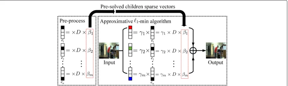
an example in Fig. 1 to express the core intuition of the algorithm. As shown in the left part, the sparse solutions of the basis vectorsem are defined as the children sparse

vectorsβ_mwhich will be employed to accelerate the pro-posed algorithm. For an input, it can also be separated into the similar patterns which have a linear relation γ with the base patterns. The sparse solution of the input is boiled down to the linear combination of the chil-dren sparse vectors. The iterative process in conventional 1-min algorithms is simplified to linear operation.

Similarly, a given signaly ∈ Rmcan be separated as a linear combination of basis functionsei∈Rmas follows:

y=γ1e1+ · · · +γiei+ · · ·γmem, (2)

where γi is the projection of yoverei. The selection of

ei varies, andy can be separated into a variety of base

patterns. The only criterion of basis selection is the inde-pendency of each basis, i.e., the bases must span the entire

space ofy. In this paper, we employ the simplest type ofei,

i.e., the identity basis vectors:

ei=

0, 0,· · ·, 1

i,· · ·, 0, 0

T

, (3)

where the projectionγiofyovereiis the pixel value ofy

at siteiin the problem of image or video processing. Eachei can be regarded as the observed signal in the

unconstrained problemPλ, and we can therefore convert Eq. (1) as follows:

Pe_λ: βˆ_i=arg min

βi

λβi₁+

1

2ei−Dβi

2 2

, (4)

whereβ_iis the sparse coefficient ofeiand is defined as the

children sparse vector. In this paper, we solve the problem

P_λewith the Bregman iterative algorithm [15]. For the same size signals, Eq. (4) only need to be solved one time.

It has been determined that most data can be classified as multi-modal data composed of irrelevant subcompo-nents, for example, imaging data obtained from neuro-biology are typically composed of neuron soma, cones, and rod cells [6]. Besides [6], Donoho and Huo [28] have suggested that the selection of distinct bases that are adapted to different subcomponents will facilitate separa-tion. Inspired by [6] and [28], we assume that the sparse solutionαofycan be separated into a linear combination of its children sparse vectorsβ_ias follows:

α≈γ1β1+ · · · +γiβi+ · · ·γmβm. (5)

For a given problem or application, once the size of the processing signal is decided,ei is also known. Then, we

can pre-solve the children sparse vectorβ_i in Eq. (4) by an existing1-min algorithm. The sparse solutionαof a

new signalycan be rapidly estimated by Eq. (5) where the weightsγiis the value ofyat sitei. The iterative process in

Fig. 1Diagram of the proposed approximative1-min algorithm. An example to express the core intuition of the proposed approximative1-min

existing1-min algorithms is replaced by simple addition

and multiplication operations.

An important question remains concerning the numer-ical distance between the sparse solution of an existing 1-min algorithm and the proposed algorithm. The

dis-tance is, in fact, acceptable for many applications that demand a compositive result (e.g., foreground detection or recognition), but not for applications that expect the highest quality result possible (e.g., image deblurring or denoising). If tolerable in a specific application, the pro-posed 1-min algorithm can be used as an acceleration

engine, which can dramatically improve the computa-tional efficiency. The numerical error between the solu-tion of an existing1-min and the proposed algorithm and

the computational burden will be discussed in detail in Section 4.1.

3.2 Proposed sparse-based BGS

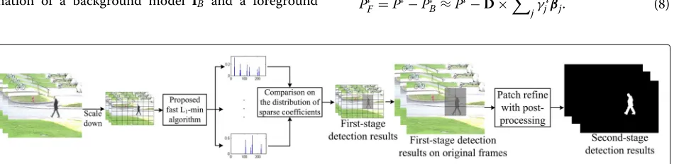
This section provides details of the proposed BGS method, and an overview of the proposed method is shown in Fig. 2. For greater completion efficiency and accuracy, we first separate the input image sequence into small patches and then scale down the resolution. Similarly, the sub-sampled images are divided into the same number patches as the original resolution. The low-resolution frames are subsequently projected over a pre-learned dictionary with the proposed fast 1-min

algorithm. Rather than casting the foreground detection as a sparse error estimation problem [9], we employ a comparison between the background and foreground which based on the distribution of sparse coefficients.

According to the sparse coefficients, we can pick up the patches that contain the foreground object. The selected patches of sub-sampled images correspond the same posi-tion of the original frames. For eliminating the inaccurate results caused by image patches, a second-stage of patch refinement is applied to the region determined in the first stage to obtain the final foreground detection.

3.2.1 Background model

The BGS problem is usually formulated as a linear com-bination of a background model IB and a foreground

candidate IF. In the existing sparse-based BGS [8–10],

the background model is regarded as a linear combina-tion of the diccombina-tionary while the diccombina-tionary is simple the combination of previous frames. However, this strategy is impractical for real-time implementation when image size becomes large. Therefore, in the present study, the origi-nal image sequence is first scaled-down with a 4:1 ratio. Then, each low-resolution frame I is detached into N

non-overlapping patches{Pi|i= 1, 2,· · ·,N}(see Fig. 2). For each patch Pi, the background model Pi_B can be formulated as follows:

Pi_B=Dαi, (6)

whereαi is the sparse coefficient andDis a pre-learned

and overcompleted dictionary.

Compared with traditional methods of obtaining bases such as wavelet and PCA, overcompleted dictio-nary learning does not emphasize the orthogonality of bases. Thus, its representation of the signal has better adaptability and flexibility. In this paper, the dictionary

D is pre-learned by the algorithm in [29] with a natural image training set. This paper constructs the training set with some images that contains nature scenes. The images for foreground detection do not include dictionary train-ing set. The traintrain-ing images are separated as the same size as the patchesPi. We set the regularization parameter in [29] as 1.2/KwhereK×Kis the size ofPi. In this paper,D

is global and suitable for arbitrary scenes, which indicates that, onceDis learned, it can be employed for any testing dataset.

Before solving the sparse coefficientsαi, we construct

the image basisein Eq. (3) of the same size asPiand obtain

the children sparse vectorsβofe. Then, the background modelP_Bi in Eq. (6) can be rewritten as follows:

Pi_B=Dαi≈D×

jγ i

jβj, (7)

whereγ_jiare the projection coefficients ofP_Bi overej. For

a patchPiof the current frameI, the foreground patchPi_F

is formulated as follows:

Pi_F =Pi−Pi_B≈Pi−D×

jγ i

jβj. (8)

Fig. 2Proposed BGS method. We first scale down the resolution of the original image sequences. The sub-sampled frames are subsequently projected over a pre-learned dictionary with the proposed1-min algorithm. Then, we employ a comparison based on the distribution of the sparse

Actually, no matter how precise Pi_B is, it cannot com-pletely predict the state of the next frame. As such, a slight difference exists between the current frame patch

Piand the background modelP_Bi, which can lead to false detection. To avoid differences caused by dynamic tex-tures or signal noise, we project the current frame patchPi

over the pre-learned dictionaryDand compute the sparse coefficientα. Then, Eq. (8) is converted as follows:

Pi_F=Dα−Dα≈D×

jγ

_i

j βj−D×

jγ i jβj

=D×

j

γi

j −γji βj, (9)

where γ_ji are the projection coefficients of the current frame patchPiover the basisej.

3.2.2 First-stage foreground detection

As described in Section 1, we apply the distribution of sparse coefficients rather than the sparse error to estimate the foreground. This is done because the appearance of the foreground in the scene will cause changes in the pro-jection ofPi_BoverD. In other words, when a current frame containing moving objects is presented by the subspace spanned by pure background bases, the unchanged area of the scene can be recovered. In contrast, the changed area is reconstructed according to the deviation in the projec-tion on the subspace. Measuring this deviaprojec-tion satisfies the purpose of foreground detection. In the first stage, or low-resolution stage, the region where a foreground may exist can be detected as follows:

⎧ ⎪ ⎪ ⎪ ⎨ ⎪ ⎪ ⎪ ⎩

1(i)= jγ

_i

j βj−

jγjiβj 1

jγjiβj 1

,

2(i)= jγ

_i

j βj 0−

jγjiβj

0

jγjiβj 0

,

(10)

whereirepresents theith patch ofIand1(i)and2(i)

are the differences in the distributions and values of the sparse coefficients between the current patchDαand the background modelDαin Eq. (9). Due to adoption of iden-tity basis vectors as basis functions ej, γji equals to the

pixel value of theith patch at sitej.

Given that the distributions and values of the sparse coefficients reflect which subspace is expanded by the test frame, we can use these parameters to determine whether a monitored scene has moving content. Specifi-cally, an unchanging image content tends to have identical distributions and corresponding values. In contrast, if a foreground object enters the scene and changes the con-tent, it generates distinct distributions and values for the sparse coefficients.

To facilitate the detection operation, we combine1(i)

and2(i)as follows:

(i)=μ11(i)+μ22(i), (11)

whereμ1 andμ2are the unitary parameters that

deter-mine the respective weights of1(i)and2(i). Because

the1-norm, or least absolute deviation, can better

repre-sent the distribution of the sparse coefficient and ensure a more distinguishable difference,μ1is set to a relatively

large value (0.60–0.75) as the dominant weight, whileμ2

is smaller (0.25–0.40).

The first-stage detection results in the original resolu-tion by different criteria are shown in Fig. 3. We employ 1and2, respectively, to segment the foreground which

are shown in Fig. 3c, d. We can find that the results by 1are more accurate. However, some foreground patches

(the book in the first row) are missed by1. Though the

results by2have more false-positive pixels, they can still

complement the detection results by 1. Therefore, we

combine1and2in Eq. (11) to obtain a better result as

shown in Fig. 3e. However, the results by Eq. (11) are still rough and inaccurate. A second-stage refinement should be performed.

3.2.3 Second-stage foreground detection

We denote the foreground patches detected by the first-stage in original frameIas{PF_t ∈ RK×K_{|t= 1, 2,· · ·,n}.}

For each patchPF_t shown by the green squares in Fig. 4, we use a smaller L × L sliding window shown by the blue square on the right-hand side of Fig. 4 to determine whether the central pixel in red belongs to the foreground. Similar to the process employed in the first stage, we train a new dictionaryDwhose atoms have the dimensionL2. Equations (9–11) are again employed, and the difference valuesin Eq. (11) are obtained for eachL×L patch. To acquire a more precise result, we further processas follows:

=+

k∈neighbor()

(k), (12)

where neighbor()defines a neighborhood patch of the current sliding window, as shown by the black square on the right-hand side of Fig. 4.

Equation (12) enhances the effect of segmentation because the question of whether a pixel belongs to a fore-ground object depends not only on its own intensity but also on the intensities of its neighborhood regions. As shown in Fig. 3d, patch-wise refinement based on first-stage detection achieves far more precise results, where the resulting foreground outlines show good agreement with the ground truth results shown in Fig. 3b.

3.2.4 Background update

Fig. 3Two-stage foreground detection.aFrames extracted from the Office [38], Water surface [30], and Skating [38] datasets.bGround truth. cFirst-stage detection results by1.dFirst-stage detection results by2.eFirst-stage detection results by.fSecond-stage detection results by

proposed BGS method

in our work is learned as a pre-processing step employ-ing arbitrary images, the update process of background

P_Bi requires updating the sparse coefficients αi of the

background model every frame or after some number of frames according to the implementation requirements. The updating strategy of the background model is given as follows:

αi+1=(1−ρ)αi+ραi, (13)

whereαiandαiare the sparse coefficients of background

model P_Bi and current image patchPi, respectively, and ρ∈[ 0.2, 0.5] is the learning rate.

In the proposed method, we initialize the background model with the first several frames and update only the sparse coefficients of the image patches that are distin-guished as background. In other words, if theith image patchPi_{belongs to the foreground, the proposed method}

does not update the corresponding sparse coefficient αi

of the background model. We evaluate the performance of the background update. The dataset Airport [30] with a stationary person is selected. As shown in Fig. 5a, a

person remains stationary. The initialization data of Air-port which is free from foreground objects is not available. The updated background images are shown in Fig. 5b. When an object remains stationary, the proposed method will regard it as a background as shown the first two rows of Fig. 5. When the object starts to move again, it will be formulated as a foreground as shown in the last row of Fig. 5. Benefiting from the power of sparse represen-tation, the simple update rule in Eq. (13) can obtain a proper background model for foreground detection. This is because that sparse coefficients are more robust and effective than the pixel intensity. The overall BGS method is described in Algorithm 1.

4 Experimental results and discussion

To evaluate the performance of the proposed method, the experimental study was divided into two parts: one part tested the proposed approximative1-min algorithm and

the other part tested the proposed BGS method. All exper-iments are performed using MATLAB on a laptop with a 2.50-GHz Intel Core i7-4710MQ processor and 16 GB of memory.

Fig. 5Background updating.aImage sequences with a stationary person.bThe updated background.cThe detection results

4.1 Performance of the proposed approximative1-min algorithm

In the first experiment, we compared the performance of solving the problemP1orPλby eight1-min algorithms

including gradient projection for sparse reconstruction (GPSR) [31], SPGL1-Lasso [32], orthogonal matching pur-suit (OMP) [33], subspace purpur-suit (SP) [34], DGS [8], the Bregman iterative algorithm [15], l1-ls [35], and the proposed approximative1-min algorithm.

We randomly generated a one-dimensional (1D) sparse signal with values ±1, where the dimension n of the signal αwas 256. The observation matrixDwas gener-ated by am×nmatrix with independent and identically distributed (i.i.d.) elements derived from a Gaussian dis-tribution N(0, 1), and each row in the matrix was nor-malized to a unit magnitude. The recovery error and running time were introduced for quantitative evalua-tion. The recovery error is defined as the difference between the estimated signal αˆ and the ground truth α: αˆ−α₂/α2. A comparison of the recovery error and running time performances of the eight1-min

algo-rithms is shown in Fig. 6 with respect to a changing number of measurementsm. To reduce the randomness, we repeat the experiment 100 times for each measurement number plotted in Fig. 6. With respect to the recovery error shown in Fig. 6a, the Bregman iterative algorithm [15] demonstrates the best performance while GPSR [31], SPGL1-Lasso [32], l1-ls [35], and the proposed method perform similarly and can be classified as the second performance tier. Relative to initial reports [8], the per-formance of DGS is sub-par because the simulated signal

has no distinct grouping trend. Fig. 6b shows that the proposed method consumes the least computation time of all methods considered regardless of the measurement number employed. The experimental results shown in Fig. 6 verify that the proposed approximative1-min

algo-rithm can achieve competitive solutions with less com-plexity and reduced computational time for real-time BGS implementation.

To visually represent the performance of the eight1

-min algorithms, we applied these algorithms to the two-dimensional (2D) Lena image I (256× 256), as shown in Fig. 7. The image was detached into non-overlapping 8 × 8 patches. The dictionary D ∈ R64×256 was pre-learned [29] with 256 atoms. The recovery error is defined as the difference between the recovery image Dαˆ and the original imageI:Dαˆ −I₂/I2. Figure 7a–h show the recovered Lena image (above) and the recovery error (below) by GPSR [31], SPGL1-Lasso [32], OMP [33], SP [34], DGS [8], the Bregman iterative algorithm [15], l1-ls [35], and the proposed approximative1-min algorithm,

respectively. Although the recovered result is not the best, the proposed approach significantly accelerates the pro-cessing of the solution with least time, and as shown in Fig. 7, the difference between the results of the proposed method and those of the other methods is scarcely recog-nizable to the human eye, which indicates that the results of the proposed method are sufficiently accurate for the BGS problem. As described in Section 3.1, the numeri-cal distance is tolerable for BGS, and the proposed1-min

Fig. 6Recovery results with different measurement numbers.aThe recovery error.brunning time

Algorithm 1:Proposed BGS algorithm

Input : Image sequenceI1,I2,· · ·,IM.

Output: The binary foregroundIF₁,IF₂,· · ·,IF_M.

Initialization:

1 Compute the children sparse vectorβ.

2 Scale down the original sequence with a four to one

ratio:I₁,I₂,· · ·,I_M.

3 Detach each frameI_mintoNnon-overlapping

patches:P1_m,P2_m,· · ·,PN_m.

4 Initialize the background model P_Bi =Pi₁≈D×_jγ_jiβj,i∈[ 1,· · ·,N].

End initialization

5 form←2toMdo

6 fori←1toNdo

7 compute the foreground differencePmi_F using

Eq. (9);

8 detect the foreground region using Eqs. (10)

and (11);

9 ifPmiis detected as a foreground regionthen

10 refine the corresponding region inI_musing

Eq. (12);

else

11 update background modelPmi_B using

Eq. (13);

4.2 Performance of the proposed BGS algorithm

This section evaluates the performance of the proposed BGS method and is divided into two parts: qualitative and quantitative evaluation. All tested videos are 160×128. The dictionary sizes in the two-stage foreground detec-tion are 8×8 pixels with 256 atoms in the first stage and 3×3 pixels with 256 atoms in the second stage. We quali-tatively and quantiquali-tatively compare the proposed method with classic BGS algorithms including SOBS [5], ViBe [36], and SuBS [2], as well as the sparse and low-rank model of Xiao et al. [17], DECOLOR [22], MAMR [24], RePROCS [37], and GOSUS [27]. For all algorithms, we adjusted parameters to obtain what appeared to be optimal results on the tested dataset.

4.2.1 Qualitative evaluation

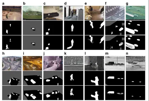
Movement in captured scenes can be divided into two parts. One part represents the foreground, which is an independent object that has no relationship to the scene. The other part is periodical or irregular, such as rain, snow, waves, and moving trees, and should be classi-fied as the background based on its relevance to the scene. Therefore, an ability to distinguish the two types of movement becomes an important criterion for motion detection. In this section, we conduct experiments on real-image sequences from the I2R dataset [30] and CDnet dataset [38].

Fig. 7Comparison of recovered results with different1-min algorithms. The recovered Lena image (above) and the error (below) byaGPSR [31], bSPGL1-Lasso [32],cOMP [33],dSP [34],eDGS [8],fthe Bregman iterative algorithm [15],gl1-ls [35], andhthe proposed approximative1-min

We compared various motion detection approaches with the proposed method for the diverse dynamic scenes shown in Fig. 8a, where the ground truth BGS results are shown in Fig. 8b. The testing frames are extracted from the Curtain [30], Water Surface [30], Fountain [30], Fountain02 [38], Snow fall [38], and Skating [38] datasets, which include different types of periodical or irregular background motion such as a curtain blown by the wind, flowing water, or falling snowflakes. The first row contains a background subject to changes caused by the motion of a curtain, and the foreground consists of a moving person wearing a white shirt that is similar to the background. As shown in the top row of Fig. 8c, the proposed method detects the foreground well and is robust with respect to the curtain motion. The second row presents the same results with a fluctuating water surface.

SuBS [2] can handle the dynamic background well and generate robust detection results. Due to the post-process in SuBS, the results seem to be overly smooth. Similarly, DECOLOR [22] method has the same problem because the single regularized parameter cannot adequately dis-tinguish the low-rank part (background) from the sparse error part (foreground). The Fountain and Fountain02 sequences present another form of non-stationary back-ground. The results of SOBS [5] and the proposed method manage these conditions well. However, the floating water leads to false-positive results of Vibe [36], MAMR [24], and RePROCS [37]. Weather variations such as rain and

snow, which can be regarded as an irregular background motion, are also a challenge for BGS. The Snow fall and Skating datasets reflect this situation. However, the low-rank model GOSUS [27] cannot detect the left person in Skating due to the falling snow. The proposed method effectively eliminates the influence of the dynamic tex-tures, and accurately detect the foreground. More dis-cussion about the models comparison is shown in the following section.

4.2.2 Quantitative evaluation

The quantitative performance of the algorithms is evalu-ated at the pixel level. Three different quantitative metrics, namely, Recall, Precision, and F-measure, were adopted. The three metrics are defined as follows [5].

Recall= tp

tp+fn. (14)

Precision= tp

tp+fp. (15)

F−measure= 2×RecallPrecision

Recall+Precision]. (16) Here,tpis the number of pixels correctly classified as the foreground, whereastp+fnandtp+fpare the number of pixels detected as foreground pixels by the ground truth and the proposed method, respectively. Therefore, Recall and Precision denote the percentage of detected true

positives as compared to the total number of true posi-tives in the ground truth and the total number of detected pixels in the proposed method. Because Recall and Preci-sion conflict to each other, we employ the F-measure as the primary metric in the quantitative evaluation.

The CDnet [38] datasets are much larger and more abundant that any of the other datasets and include suffi-cient ground truth data for quantitative evaluation. There-fore, as listed in Table 1, we selected eighteen datasets from nine categories on the CDnet website, includ-ing baseline, dynamic background, intermittent object motion, shadow, thermal, bad weather, low frame rate, night videos, and turbulence. The quantitative results of the nine categories are listed in Table 1. We present the average frames per second by each method as shown in Table 2. In addition to the datasets employed in the above section, we present the results of 14 additional datasets obtained from CDnet [38] in Fig. 9. The third and sixth rows of Fig. 9 are the detection results of the proposed BGS method.

It is noted that the proposed BGS method obtained the best average F-measure compared to all other methods while SuBS [2] ranks second. Compared to the proposed method, SuBS [2] is sensitive to the Turbulence dataset due to the flow distortion. Besides, DECOLOR [22] has a good performance on F-measure while the frames per

second (fps) processed by DECOLOR [22] (MATLAB implementation) is only 2.3. The proposed method can achieve 29.3 fps while this number of MAMR (MATLAB implementation) is about 3.6. This accelerated processing speed is possible because the proposed method replaces an iterative optimization by linear addition and multipli-cation operations. For the baseline category (Office and PETS2006 datasets), the performances of all methods con-sidered are acceptable. For the Fountain01 dataset, all the methods failed because the fountain movement exceeds the background updating capabilities of the methods. In contrast, the movement of Fountain02 is smooth and con-tinuous, and SOBS [5] and SuBS [2] both perform well. The proposed method demonstrates competitive results for the thermal and turbulence categories (Park, din-ing room, turbulence0 and turbulence3 datasets). This is because the datasets of these two categories present dis-tinct irregular fluctuations similar to noise that cannot be formulated by a mathematical expression. The proposed method employs sparsity over a pre-learned dictionary that can restrain this condition. The fps performance of low-rank methods such as RePROCS [37] and GOSUS is poor. This is because that the iterative pursuit of low-rank matrix or sparse matrix is time-consuming. The pro-posed approximative1-min algorithm avoid the iterative

process and employ the power of sparse representation.

Table 1The quantitative F-measure metric (%) of the compared BGS methods on CDnet [38] datasets

Dataset Classic methods Low-rank methods Sparse methods

SOBS ViBe SuBS DECO MAMR GOSUS RePROCS Xiao Proposed

Office 96.63 90.32 97.02 95.34 85.23 91.54 90.87 89.61 94.31

PETS2006 85.26 84.32 85.12 79.13 77.63 78.21 79.33 75.16 86.16

Fountain01 11.21 6.05 15.63 2.71 6.35 7.55 8.36 7.15 8.61

Fountain02 85.81 63.38 84.69 75.36 77.65 70.23 67.93 78.38 83.44

Parking 36.68 45.33 72.76 34.61 58.03 30.84 40.37 59.71 75.31

Sofa 62.18 61.97 62.69 50.31 63.46 51.24 47.87 67.49 69.63

Cubicle 72.05 79.65 79.33 77.67 69.38 71.23 69.34 70.91 73.64

Copy Machine 57.21 81.71 89.74 78.18 70.68 79.22 74.32 69.61 75.61

Park 59.70 69.53 58.69 75.81 70.96 72.33 66.98 70.14 74.73

Dining Room 71.73 75.49 70.36 82.47 78.33 76.48 70.38 72.30 84.67

Snow fall 67.01 82.49 85.03 83.46 82.36 81.84 76.70 73.41 85.27

Skating 76.33 73.67 80.25 83.81 85.68 79.83 75.93 78.64 82.11

Tram Crossroad 74.18 85.64 71.36 74.62 76.69 75.65 67.33 71.49 75.29

Turnpike 78.98 90.64 89.67 88.37 85.44 85.45 79.43 79.61 86.82

Winter Street 51.04 30.58 55.56 66.13 49.64 38.45 33.20 57.91 60.34

Tram Station 71.32 70.69 72.91 69.54 70.03 72.98 68.26 61.41 76.17

Turbulence0 2.64 5.36 8.65 38.34 35.67 37.94 33.62 29.34 40.34

Turbulence3 74.96 65.48 80.28 77.67 81.36 68.29 59.33 79.56 87.64

Average 63.05 64.57 69.98 68.53 68.03 64.96 61.64 66.21 73.33

Table 2Average frames per second (FPS) of each method

Dataset Classic methods Low-rank methods Sparse methods

SOBS ViBe SuBS DECO MAMR GOSUS RePROCS Xiao Proposed

FPS 28.5 31.9 48.7 2.3 3.6 0.54 0.78 2.6 29.3

Platform C++ C++ C++ MATLAB MATLAB MATLAB MATLAB MATLAB MATLAB

5 Conclusions

Sparse and low-rank model based BGS applications and methods have received considerable attention. However, the iterative optimization process used to obtain sparse or low-rank solutions is computationally expensive. This paper proposed the approximative 1-min algorithm to

provide a level of computational efficiency unobtainable by previous sparse model based approaches. Moreover, the proposed approach employed the sparsity rather than the sparse error to detect the foreground, which has been proven effective and robust to dynamic and corrupted scenes.

However, this work is at a preliminary stage. For exam-ple, how the signal should be separated into basic atoms

ei remains an open question, even though a satisfactory

result can be obtained in separating the signal using the simplest method, as demonstrated in Eq. (3) by this work. Another future work is to measure the numerical differ-ences of the sparse solution between the proposed1-min

method and existing1-min algorithms. The difference is

acceptable for motion detection, but this does not ensure it can be used for other applications. Thus, mathemati-cally defining this difference is required to determine the potential of the proposed algorithm.

Acknowledgements

This research was partially supported by National Natural Science Foundation (NSFC) of China under project No. 61403403 and No. 61402491.

Authors’ contributions

HX carried out the main part of this manuscript. YL participated in the design of the approximative1-min algorithm. MZ participated in the discussion. All authors read and approved the final manuscript.

Competing interests

The authors declare that they have no competing interests.

Received: 29 June 2016 Accepted: 30 November 2016

References

1. T Bouwmans, Traditional and recent approaches in background modeling for foreground detection: An overview. Comput. Sci. Rev.11, 31–66 (2014) 2. P St-Charles, G Bilodeau, R Bergevin, Subsense: a universal change

detection method with local adaptive sensitivity. IEEE Trans. Image Process.24(1), 359–373 (2015)

3. C Stauffer, WEL Grimson, inProceedings of the IEEE Comput. Vis. Pattern Recognit. (CVPR). Adaptive background mixture models for real-time tracking (IEEE, Ft. Collins, 1999), pp. 246–252

4. NM Oliver, B Rosario, AP Pentland, A Bayesian computer vision system for modeling human interactions. IEEE Trans. Pattern Anal. Mach. Intell.22(8), 831–843 (2000)

5. L Maddalena, A Petrosino, A self-organizing approach to background subtraction for visual surveillance applications. IEEE Trans. Image Process. 17(7), 1168–1177 (2008)

6. YC Eldar, G Kutyniok (eds.),Compressed Sensing: Theory and Applications (Cambridge University Press, Cambridge CB2 8RU, 2012)

7. V Cevher, A Sankaranarayanan, MF Duarte, D Reddy, RG Baraniuk, R Chellappa, inProceedings of the European Conf. Comput. Vis. (ECCV). Compressive sensing for background subtraction (Springer, Marseille, 2008), pp. 155–168

8. J Huang, X Huang, D Metaxas, inProceedings of the IEEE Int. Conf. Comput. Vis. (ICCV). Learning with dynamic group sparsity (IEEE, Kyoto, 2009), pp. 64–71

9. R Sivalingam, D Alden, B Michael, M Roland, V Morellas, N

Papanikolopoulos, inProceedings of the IEEE Int. Conf. Rob. Autom. (ICRA). Dictionary learning for robust background modeling (IEEE, Shanghai, 2011), pp. 4234–4239

10. C Zao, X Wang, W-K Cham, Background subtraction via robust dictionary learning. EURASIP J. Image Video Process, 1–12 (2011)

11. M Osborne, B Presnell, B Turlanch, A new approach to variable selection in least squares problems. IMA J. Numer. Anal.20(3), 389–404 (2000) 12. B Efron, T Hastie, I Johnstone, R Tibshirani, Least angle regression. Ann.

Stat.32(2), 407–499 (2004)

13. J Friedman, T Hastie, R Tibshirani, Pathwise coordinate optimization. Ann. Appl. Stat.1(2), 302–332 (2007)

14. E Hale, W Yin, Y Zhang, A fixed-point continuation method for1 regularized minimization with applications to compressed sensing. CAAM TR07-07, Rice University.43, 1–44 (2007)

15. W Yin, S Osher, D Goldfarb, J Darbon, Bregman iterative algorithms for compressed sensing and related problems. SIMA J. Imag. Sci.1(1), 143–168 (2008)

16. G Xue, L Song, J Sun, Foreground estimation based on linear regression model with fused sparsity on outliers. IEEE Trans. Circ. Syst. Video Technol. 23(8), 1346–1357 (2014)

17. H Xiao, Y Liu, S Tan, J Duan, M Zhang, A noisy videos background subtraction algorithm based on dictionary learning. KSII Trans. Internet Inf. Syst.8(6), 1946–1963 (2014)

18. T Bouwmans, E Zahzah, Robust PCA via principal component pursuit: a review for a comparative evaluation in video surveillance. Comp. Vision Image Underst.122, 22–34 (2014)

19. C Qiu, N Vaswani, inProceedings of the IEEE Communication, Control, and Computing. Real-time robust principal components’ pursuit (IEEE, Tamil Nadu, 2010), pp. 591–598

20. E Candès, X Li, Y Ma, J Wright, Robust principal component analysis? J. ACM.58(3), 1–37 (2011)

21. X Cui, J Huang, S Zhang, D Metaxas, inProceedings of the European Conf. Comput. Vis. (ECCV). Background subtraction using low rank and group sparsity constraints (Springer, Firenze, 2012), pp. 612–625

22. X Zhou, C Yang, W Yu, Moving object detection by detecting contiguous outliers in the low-rank representation. IEEE Trans. Pattern Anal. Mach. Intell.35(3), 597–610 (2013)

23. P Rodríguez, B Wohlberg, inProceedings of the IEEE Image Processing. A Matlab implementation of a fast incremental principal component pursuit algorithm for video background modeling (IEEE, Paris, 2014), pp. 3414–3416

24. X Ye, J Yang, X Sun, K Li, C Hou, Y Wang, Foreground-background separation from video clips via motion-assisted matrix restoration. IEEE Trans. Circ. Syst. Video Technol.25(11), 1721–1734 (2015)

25. J He, L Balzano, A Szlam, inProceedings of the IEEE Comput. Vis. Pattern Recognit. (CVPR). Incremental gradient on the Grassmannian for online foreground and background separation in subsampled video (IEEE, Boston, 2012), pp. 1568–1575

26. F Seidel, C Hage, M Kleinsteuber, pROST—a smoothed Lp-norm robust online subspace tracking method for realtime background subtraction in video. Mach. Vis. Appl.122, 1–13 (2013)

27. J Xu, V Ithapu, L Mukherjee, JM Rehg, V Singh, inProceedings of the IEEE Int. Conf. Comput. Vis. (ICCV). Gosus: Grassmannian online subspace updates with structured-sparsity (IEEE, Sydney, 2013), pp. 3376–3383

28. D Donoho, X Huo, Uncertainty principles and ideal atomic decomposition. IEEE Trans. Inf. Theory.47(7), 2845–2862 (2001) 29. J Mairal, F Bach, J Ponce, G Sapiro, Online learning for matrix factorization

and sparse coding. J. Mach. Learn. Res.11, 19–60 (2010) 30. L Li, W Huang, IYH Gu, Q Tian, Statistical modeling of complex

backgrounds for foreground object detection. IEEE Trans. Image Process. 13(11), 1459–1472 (2004)

31. M Figueiredo, R Nowak, S Wright, Gradient projection for sparse reconstruction: application to compressed sensing and other inverse problems. IEEE J. Sel. Top. Sign. Process.1(4), 586–597 (2007)

32. E Berg, M Friedlander, Sparse optimization with least-squares constraints. SIAM J. Optim.21(4), 1201–1229 (2011)

33. J Tropp, A Gilbert, Signal recovery from random measurements via orthogonal matching pursuit. IEEE Trans. Inf. Theory.53(12), 4655–4666 (2007)

34. D Wei, M Olgica, Subspace pursuit for compressive sensing signal reconstruction. IEEE Trans. Inf. Theory.55(5), 2230–2249 (2009) 35. S-J Kim, K Koh, M Lustig, S Boyd, D Gorinevsky, An interior-point method

for large-scale l1-regularized least square. IEEE J. Sel. Top. Sign. Process. 1(4), 606–617 (2007)

36. O Barnich, MV Droogenbroeck, Vibe: A universal background subtraction algorithm for video sequences. IEEE Trans. Image Process.20(6), 1709–1724 (2011)

37. H Guo, N Vaswani, C Qiu, inProceedings of IEEE Global Signal and Information Processing. Practical ReProcs for separating sparse and low-dimensional signal sequences from their sum—part 2 (IEEE, Atlanta, 2014), pp. 369–373