Exponentially Fitted 2 Step Simpson’s Method for Oscillatory/Periodic Problems

http://dx.doi.org/10.4236/jamp.2016.42043

Exponentially-Fitted 2-Step Simpson’s

Method for Oscillatory/Periodic Problems

Ashiribo Senapon Wusu, Bosede Alfred Olufemi, Akanbi Moses Adebowale

Department of Mathematics, Lagos State University, Lagos, Nigeria

Received 15 December 2015; accepted 23 February 2016; published 26 February 2016

Copyright © 2016 by authors and Scientific Research Publishing Inc.

This work is licensed under the Creative Commons Attribution International License (CC BY).

http://creativecommons.org/licenses/by/4.0/

Abstract

Following a six-step flow chart, exponentially-fitted variant of the 2-step Simpson’s method suita-ble for solving ordinary differential equations with periodic/oscillatory behaviour is constructed. The qualitative properties of the constructed methods are also investigated. Numerical experi-ments on standard problems confirming the theoretical expectations regarding the constructed methods compared with other existing standard methods are also presented. Our results unify and improve the existing classical 2-step Simpson’s method.

Keywords

Exponentially-Fitted, Simpson Method, Oscillatory, Periodic, ODE

1. Introduction

In this paper, we consider the first-order initial value problem of the form

( )

, ,

[

0,

]

,

( )

0 0

u′ = f t u t∈ t T u t =

η

(1) with oscillatory/periodic solution.

encountered in fields like mechanics, electronic, astrophysics, chemistry and engineering. The idea of using exponentially fitted formulae for differential equations was first proposed by Liniger and Willoughby [9]. Integration formulae containing free parameters were derived and these parameters were chosen so that a given function exp

( )

q where q was real, satisfied the integration formulae exactly. This was tested on linear multistep method for k=1, however Jackson and Kenue [10] derived a fourth order exponentially fitted formulae based on a linear 2-step formula and were A-stable. Based on this idea, Cash [11], in his own work, attempted using Multiderivative Linear Multistep Method (MLMM) with k = 1 in the second derivative formulae. Particular Runge-Kutta (RK) algorithms have been proposed by several authors [12]-[15] in order to solve this class of problems. Vanden Berghe et al.[16] [17] on the other hand, introduced other exponentially fitted RK (EFRK) methods which integrate exactly first-order systems whose solutions can be expressed as linear combinations of functions of the form

{

exp

( )

λt , exp

(

−λt

)

}

or

{

cos

( )

ωt , sin

( )

ωt

}

.

Here, we analyze the construction and implementation of the exponentially-fitted variants of the 2-step Simpson method for solving problems of the form (1) which possess oscillatory/periodic solution, taking into account the six-step flow chart described by Ixaru and Vanden Berghe in [6].

The main interest of this work is to modify the classical 2-step Simpson method for adaptation to oscillatory/ periodic problems.

2. Construction of Method

The classical 2-step Simpson method for solving (1) is given by

(

)

1 1 1 4 1 .

3

n n j j j

h

u₊ =u₋ + f ₊ + f + f ₋ (2) To begin the construction of the exponentially-fitted variants of (2), we rewrite (2) in a more general way as

(

)

1 0 1 2 1 1 0 1 .

n n j j j

u+ =α u− +h β f + +β f +β f− (3)

Following the six-step flow chart, the corresponding linear difference operator 

[ ]

h a, reads

[ ]

h a u t,

( )

=u t

(

+h

)

−α0u t

(

−h

)

−h(

(

β2u t′

(

+h

)

+β1u t′

( )

+β0u t′

(

−h

)

)



where a:=

(

α β β β

₀, ₀, ₁, ₂

)

where a:=

(

α β β β

₀, ₀, ₁, ₂

)

. Applying step II of the six-step procedure, the resulting system of equations is compatible when M =5. Solving the resulting system, we have

0 0 2 1

1 4

1, ,

3 3

α = β =β = β = (4) which are the coefficients of the classical method (2).

Applying step III, we find that

(

,

) (

0 2

)

sinh

( )

(

0 1 cosh

)

( )

G+ Z a = β −β Z Z − α − Z (5)

(

)

(

0

)

( )

(

)

( )

1 2 0

1 sinh

, cosh

Z

G Z a Z

Z α

β β β

− _{= − +} + _{− +}

(6) where z=

ω

h=

ω

_h and 2

Z=z , ω (the frequency of oscillation) is real or imaginary. (For the trigonometric case, i.e., ω is imaginary, choose z=

ω

h=i h

µ

, i.e. z2 = −

µ

2h2 =Z.)

To implement step IV, consider the reference set of M functions:

(

)

(

)

(

)

{

1, ,t,tK, exp ±ωt t, exp ±ωt ,,tPexp ±ωt

}

• K=2,P=0, the mixed case with the set _{1, , , expt t}2

(

_±ω_t

)

• K=0,P=1, the mixed case with the set 1, exp

(

±

ω

t t

)

, exp

(

±

ω

t

)

The coefficients of the method for each case are obtained by the implementation of step V as follows: S1:

(

K P,

) (

= 4, 1−

)

In this case, the solution is already known by (4)

S2:

(

K P,

) ( )

= 2, 0

( )

( )

(

)

( )

( )

(

)

( )

( )

(

)

0 2 2 1 0 1, sinh , cosh 1

csch cosh sinh

2 , sinh cosh 1 z z z z z

z z z

z z z z z α β β β =   − _ = _ −     _{− }      = _  − _ = _ − _ (7)

S3:

(

K P,

) ( )

= 0,1

( )

( )

( )

(

)

( )

0 2 2 1 2 0 2 1, coth 1 ,

2 cosh csch

,

coth 1

z z

z

z z z

z z z z α β β β =   − _ = _  −  = _   − = _  (8)

As expected, the exponentially fitted variants reduce to the the classical method as z→0.

3. Error Analysis: Local Truncation Error (

lte

)

The general expression of the leading term of the local truncation error (lte) for an exponentially fitted method with respect to the basis functions

(

)

(

)

(

)

{

1, ,t,tK, exp ±ωt t, exp ±ωt ,,tPexp ±ωt

}

(9) takes the form (see [6])

( ) ( )

₁

₍

₁

(

₎

( )

)

(

)

1

( )

1 2 2 1

1

1 !

P

P K

EF M K

P

a Z

lte t h D D u t

K Z ω

∗ + + + + + = − − +  (10) with K, P and M satisfying the condition K+2P=M−3.

For the three methods constructed above, one finds the following results: • S1:

(

K P,

) (

= 4, 1−

)

( )

1 5 ( )5

_{( )}

90

EF

lte t = − h u t (11) • S2:

(

K P,

) ( )

= 2, 0

( )

5

(

)

(

2 ( )3

_{( )}

( )5

_{( )}

)

0 2 0

1

3 3 1

6

EF

lte t h u t u t

Z α β β ω

= − − + −

• S3:

(

K P,

) ( )

= 0,1

( )

5

(

)

(

( )5

_{( )}

2 ( )3

_{( )}

4

_{( )}

)

0 2 1 0

2

1

1 2

EF

lte t h u t u t u t

Z α β β β ω ω ′

4. Existence and Uniqueness of Solution

The following theorem states conditions of f t u

( )

, which guarantee the existence of a unique solution of the initial value problem (1)

Theorem 1. Let f t u

( )

, be defined and continuous for all points

( )

t u, in the region  defined by

a≤ ≤t b, −∞ < < ∞u , a and b finite, and let there exist a constant  such that, for every t u u, ,  such that

( )

t u, and

( )

t u,  are both in ,

( )

,

( )

,

f t u − f t u ≤u−u (12) then if

η

₀ is any given number, there exists a unique solution u t

( )

to the initial value problem (1), where

( )

u t is continuous and differentiable for all

( )

t u, ∈. Lambert [3].

The requirement (12) is known as the Lipschitz Condition, and the constant  is called the Lipschitz constant.

This condition may be thought of as being intermediate between differentiability and continuity, in the sense that

• f t u

( )

, continuously differentiable with respect to u ∀

( )

t u, ∈ • ⇒f t u

( )

, satisfies a Lipschitz Condition w.r.t. u ∀

( )

t u, ∈ • ⇒f t u

( )

, continuous w.r.t.u ∀

( )

t u, ∈

In particular, if f t u

( )

, possesses a continuous derivative w.r.t.y for all

( )

t u, ∈, then, by the mean value theorem

( )

,

( )

, f t u

( )

,

(

)

f t u f t u u u

u ∂

− = −

∂

 

where u is a point in the interior of the interval whose end-points are u and u, and

( )

t u, and

( )

t u,  are both in . Clearly (12) is satisfied if

( )

( )

,

, sup

x u

f x u

u

∈

∂ =

∂



 (13) is chosen.

5. Contraction Mapping Theorem

In the sequel, we shall apply the following Contraction Mapping Theorem:

Theorem 2. (Contraction Mapping Theorem). Consider a set D⊂n and a function : n

g D→ . Assume

• D is closed (i.e., it contains all limit points of sequences in D) • x∈ ⇒D g x

( )

∈D

• The mapping g is a contraction on D: There exists q<1 such that

( )

( )

, :

x y D g x g y q x y

∀ ∈ − ≤ −

Then

• there exists a unique x∗∈D with g x

( )

∗ =x∗

• for any x( )0 ∈D, the fixed point iterates given by x( )k+1 :=g x

( )

( )k converges to x∗ as k→ ∞ • x( )k satisfies the a-priori extimate

( ) ( )1 ( )0

1

k

k q

x x x x

q

∗

− ≤ −

−

( ) ( ) ( )1

1

k q k k

x x x x

q

− ∗

− ≤ −

−

6. Application of the Contraction Mapping Theorem to LMM

If h is sufficiently small, implicit LMM methods also have unique solutions given h and u u₀, ,₁,u_k−1. To see this, let  be the Lipschitz constant for f. Given u_i,,u_{i k+ −1}, the value for u_{i k+} is obtained by solving the equation

(

,

)

i k k i k i k i

u₊ =h

β

f t₊ u₊ +g (14) where

(

)

(

)

1 0

constant

k

i k i j j i j j

g hβ f α u

−

+ +

=

=

∑

− (15)

That is, we are looking for a fixed point of

( )

u h kf t

(

i k,u

)

gi

φ

=

β

+ + (16)

If h

β

k <1, then φ is a contraction:

( )

u

( )

u h k f t

(

i k,u

)

f t

(

i k,u

)

h k u u

φ −φ  ≤ β + − +  ≤ β  −  (17)

So by the Contraction Mapping Fixed Point Theorem,

φ

has a unique fixed point. Any initial guess u_{i k}0+

yields a convergent fixed point iteration:

(

)

1

,

l l

i k k i k i k

u++ =hβ f t+ u+ (18)

7. Convergence and Stability Analysis

Theorem 3 (Dahlquist Theorem) The necessary and sufficient conditions for a linear multistep method to be

convergent are that it be consistent and zero-stable

Dahlquist theorem (3) holds also true for EF-based algorithms but, because their coefficients are no longer constants the concepts of consistency and stability have to be adapted.

Definition 4. An exponentially fitted method associated with the fitting space (9) is said to be of order p=M−r, (where r is the order of the differential equation to be solved) and it is consistent if p≥1.

Since M ≥1 for all the constructed schemes, the consistency requirement is satisfied. Hence, the constructed schemes are all consistent.

Definition 5. A linear s-step method is said to be weakly stable if there is more than one simple root of the polynomial equation

ρ ξ

( )

=0 on the unit circle.

To investigate the stability of (3), one applies the method to the test problems u′ =λu. Applying (3) to the above test problems, one obtains

(

)

(

)

1 0 1 2 1 1 0 1 0 1 2 1 1 0 1

n n n n n

n n n n

u u h u u u

u h u u u

α β λ β λ β λ

α λ β β β

+ − + −

− + −

= + + +

= + + + (19)

From the above, one finds that

(

1−β2h u

)

n+1−β1hun−

(

α0+β0h u

)

n−1=0, n=1, 2, (20)

where h=λh. The characteristics equation is given by

(

)

2

(

)

2 1 0 0

Definition 6. A region of stability is a region of the q--z plane, throughout which R q z

( )

, <1. Any closed curve defined by R q z

( )

, =1 is a stability boundary. Also, any interval

(

α β

,

)

of the real line is said to be the interval of stability if the method is stable for all q∈

(

α β

,

)

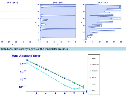
For each of the constructed methods, the region of stability is presented inFigure 1.

8. Numerical Results

Numerical experiments confirming the theoretical expectations regarding the constructed methods are now performed. The constructed methods are applied to two test problems and the result obtained compared with the classical fourth-order Taylor method, explicit four stage fourth-order Runge-Kutta method and the classical 2-step Simpson method.

8.1. Problem 1

Consider the IVP: u′ − =u t u,

( )

0 =1 with the exact solution u t

( )

=2et− −t 1. Solving the problem using different values of steplength h, the the maximum absolute errors for each steplength is obtained as presented in

Figure 2. As expected, the exponentially-fitted variants (S2:(2,0), S3:(0,1)) of the classical 2-step Simpson method performed better compared with the classical methods.

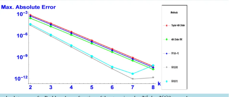
8.2. Problem 2

[image:6.595.135.538.395.705.2]

Consider the IVP: u′ =αu+eαtt u,

( )

− = −1 e−α with the exact solution u t

( )

=teαt. With α =1, the problem is solved using different values of steplength h and the maximum absolute error for each steplength is obtained as presented inFigure 3. The constructed exponentially=fitted variants also performed better compared to the classical methods.

Figure 1. Truncated absolute stability regions of the constructed methods.

Figure 2. Maximum absolute errors for Problem 1 as a function of the step-size 2 ,k 2 1 8

( )

[image:7.595.157.539.78.240.2]

Figure 3. Maximum absolute errors for Problem 1 as a function of the step-size 2 ,k 2 1 8

( )

h= − k= , α=1.

9. Conclusion

The exponentially-fitted versions of the classical 2-step Simpson method have been constructed and imple- mented in this paper. The stability and convergence properties of the constructed methods were also analysed. The results obtained from the numerical examples show that the theoretical expectations are meet (i.e. the expo- nentially-fitted variants of the classical 2-step Simpson method are suitable for solving periodic/oscillatory problems).

Acknowledgements

We thank the Editor and the referee for their comments.

References

[1] Akanbi, M.A. (2011) On 3-Stage Geometric Explicit Runge-Kutta Method for Singular Autonomous Initial Value Problems in Ordinary Differential Equations. Computing, 92, 243-263.

[2] Butcher, J.C. (2008) Numerical Methods for Ordinary Differential Equations. Wiley. http://dx.doi.org/10.1002/9780470753767

[3] Lambert, J.D. (1973) Computational Methods in ODEs. Wiley, New York.

[4] Wusu, A.S. and Akanbi, M.A. (2013) A Three-Stage Multiderivative Explicit Runge-Kutta Method. American Journal

of Computational Mathematics, 3, 121-126. http://dx.doi.org/10.4236/ajcm.2013.32020

[5] Wusu, A.S., Akanbi, M.A. and Fatimah, B.O. (2015) On the Derivation and Implementation of a Four Stage Harmonic Explicit Runge-Kutta Method. Applied Mathematics, 6, 694-699. http://dx.doi.org/10.4236/am.2015.64064

[6] Ixaru, L.G. and Vanden, B.G. (2004)Exponential Fitting Mathematics and Its Applications. Kluwer Academic Pub-lishers, 568. http://dx.doi.org/10.1007/978-1-4020-2100-8

[7] Simos, T.E. (1998) An Exponentially-Fitted Runge-Kutta Method for the Numerical Integration of Initial-Value Prob-lems with Periodic or Oscillating Solutions. Computer Physics Communications, 115, 1-8.

http://dx.doi.org/10.1016/S0010-4655(98)00088-5

[8] Vanden, B.G. and Daele, M.V. (2006) Exponentially-Fitted Stomer/Verlet Methods. Journal of Numerical Analysis,

Industrial and Applied Mathematics, 1, 241-255.

[9] Liniger, W.S. and Willoughby, R.A. (1970) Efficient Integration Methods for Stiff System of ODEs. SIAM Journal on

Numerical Analysis, 7, 47-65. http://dx.doi.org/10.1137/0707002

[10] Jackson, L.W. and Kenue, S.K. (1974) A Fourth Order Exponentially-Fitted Method. SIAM Journal on Numerical

Analysis, 11, 965-978.

[11] Cash, J.R. (1981) On Exponentially Fitting of Composite Multiderivative Linear Methods. SIAM Journal on Numerical

Analysis, 18, 808-821. http://dx.doi.org/10.1137/0718055

[12] Avdelas, G., Simos, T.E. and Vigo-Aguiar, J. (2000) An Embedded Exponentially-Fitted Runge-Kutta Method for the Numerical Solution of the Schrödinger Equation and Related Periodic Initial-Value Problems. Computer Physics Com-

munications, 131, 52-67. http://dx.doi.org/10.1016/S0010-4655(00)00080-1

(ZAMP), 30, 699-704. http://dx.doi.org/10.1007/BF01590846

[14] Coleman, J.P. and Duxbury, S.C. (2000) Mixed Collocation Methods for y′′ = f x y

( )

; . Journal of Computational and

Applied Mathematics, 126, 47-75. http://dx.doi.org/10.1016/S0377-0427(99)00340-4

[15] Franco, J.M. (2002) An Embedded Pair of Exponentially Fitted Explicit Runge-Kutta Methods. Journal of

Computa-tional and Applied Mathematics, 149, 407-414. http://dx.doi.org/10.1016/S0377-0427(02)00485-5

[16] Vanden, B.G., Meyer, H.D., Daele, M.V. and Hecke, T.V. (1999) Exponentially-Fitted Explicit Runge-Kutta Methods.

Computer Physics Communications, 123, 7-15. http://dx.doi.org/10.1016/S0010-4655(99)00365-3

[17] Vanden, B.G., Meyer, H.D., Daele, M.V. and Hecke, T.V. (2000) Exponentially-Fitted Explicit Runge-Kutta Methods.