Spatial synchronization in the human cardiovascular system

Spatial Synchronization in the Human Cardiovascular System

Aneta Stefanovska∗) and Mario Hoˇziˇc∗∗)

Group of Nonlinear Dynamics and Synergetics Faculty of Electrical Engineering, University of Ljubljana

Trˇzaˇska 25, Ljubljana, Slovenia

Concepts developed for the synchronization analysis of noisy coupled nonlinear oscillators are used to study the spatial synchronization of oscillations in the blood distribution system. We reveal that the cardiac and respiratory oscillations observed at different sites of the system are strongly phase and frequency synchronized, while the spatial synchronization of oscillations that originate locally is weaker. The results obtained support the hypothesis that the entire cardiovascular system is characterised by the same dynamics.

§1. Introduction

The human cardiovascular system distributes matter and energy to the cells and removes byproducts of their metabolism. The cells extract matter and energy from the blood which is pumped by the heart into the network of vessels. The lungs, where the blood becomes oxygenated, are also part of the cardiovascular network.

The heart of a relaxed, healthy subject, pumps an amount equivalent to the total amount of blood in the body in approximately one minute.1) Thus, in cardiovascular dynamics we consider the dynamics of blood distribution through the cardiovascular network on a time scale of around one minute. It can be characterised by the dynam-ics of the blood flow and the blood pressure in the system, and the activity of the lungs and heart pump. The function of the heart is manifested as electric potentials spread across the heart muscle, and as a mechanical pump that rhythmically expels the blood into the arterial network approximately once per second. However, the period of the heart cycle is not constant but, rather, varies in time. The frequency of respiration also varies, between 0.15 and 0.3 Hz. Consequently, the flow and the pressure change in an oscillatory fashion with time, and do so on several different time scales.

The vessel walls are not stiff: their radii continually alter, thus giving rise to a variable resistance to flow. Threeperipheralmechanisms are known to contribute to the resistance or compliance of the vessels: the intrinsicmyogenicmechanism, based on continuous contraction and relaxation of smooth muscle cells; the neurogenic

control provided by the autonomous nerve innervation of vessels; and endothelium

mediated contraction and relaxation of the vessels.2)-4) Each of these processes manifests in an oscillatory manner, and their characteristic frequencies are around 0.1, 0.04 and 0.01 Hz, respectively.

Arterial blood flow is characterised by high pressure and low resistance, and the heart frequency dominates in both the flow and pressure. Flow in veins is

characterised by low pressure and low resistance. The heart and the respiratory frequency jointly dominate in the venous flow and pressure. In the peripheral blood flow, through the capillary bed, the amplitudes of the five characteristic frequencies are all comparable in magnitude.

Although the relative amplitudes of oscillations in the blood flow differ between the two sides of the cardiovascular system, their characteristic frequencies were found to be similar, or the same, on each side of the system and for all measured sig-nals.3),5) Moreover, the heart and respiratory oscillations were recently shown to be synchronized,6)-8) the strength of phase synchronization being inversely related to the extent of respiratory modulation of the heart rate.8) At this point, new intriguing questions rise:

(i) Is each of the centrally generated oscillations — respiratory and cardiac — self-synchronized during the flow of blood through the entire network?

(ii) How are the peripherally distributed systems, such as the myogenic one, self-synchronized at different sites of the network?

§2. Synchronization and self-synchronization

Synchronization, or adjustments in time, occurs when two or more nonlinear oscillators are coupled. It appears as some relation between their phases and fre-quencies. In the classical sense, as discovered by Huygens,9) synchronization means adjustment of frequencies of self-sustained oscillations due to weak interactions. This effect is referred to asphase lockingorfrequency entrainment. Recently, the notation of synchronization has been generalised to the case of interacting noisy or chaotic oscillators (see Ref. 10) and the references therein). Phase synchronization is de-scribed as the appearance of a certain relationship between the phases of interacting systems, while in general, the amplitudes are uncorrelated.

We will use this concept in the analysis of self-synchronization of oscillations observed at different sites of the cardiovascular system.

2.1. Coupled oscillators

A subsystem of the cardiovascular system may be represented as an oscillator, described by a state vectoruwhich satisfies

du

dt =g(u,µ), (2.1)

wheregis the nonlinear rate function, andµdenotes the parameters of the oscillator. A simple limit cycle oscillator, as proposed by Poincar´e,

dxi

dt =αixi(ai−ri)−2πfiyi, dyi

dt =αiyi(ai−ri) + 2πfixi, (2.2)

and the analysis of measured time series.11) The state variables xi and yi describe

the flow and velocity of flow contributed by thei-th oscillator.

−1 0 1

−1 0 1

x

y

r

Φ

r=a

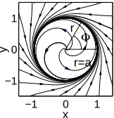
Fig. 1. The phase plane solution of Eqs. (2·2) for a basic oscillator.

Five oscillators are assumed to con-tribute to the blood flow through the cardiovascular system: cardiac, respira-tory, myogenic, neurogenicand endothe-lial related metabolic activity. Each of them is characterized by a frequency fi

and amplitude ai. The constant αi de-termines the rate at which the state vec-tor approaches the limit cycle. In polar coordinates, with radiusriand angleΦi,

the state variables are

xi =ri cosΦi, and yi=ri sinΦi. (2.3)

The system (2.2) then becomes

dri

dt =αiri(ai−ri), dΦi

dt = 2π fi. (2.4)

It has two steady-state solutions, where dri/dt = 0, at ri = 0 and ri = ai. The periodic solution travels around with period Ti = 1/fi (Fig. 1).

However, the characteristic frequencies of the cardiovascular system vary in time. Therefore, besides the autonomous part, we suppose that there also exists a com-ponent resulting from mutual interactions. Accordingly, we add a coupling term

Hi,j(xj,yj), j=i,

dxi

dt =αixi(ai−ri)−2π fiyi+εiHi,j(xj,yj), dyi

dt =αiyi(ai−ri) + 2π fixi+εiHi,j(xj,yj), (2.5)

whereεi is a coupling coefficient,Hi,j(xj,yj) represents all possible influences from

the rest of the system on thei-th oscillator. 2.2. Synchronization

In a wide sense, synchronization can be treated as the appearance of some rela-tionship between the state vectors of interacting systems. For two systems it is then the existence of a relation u2(t) =F[u1(t)]. If the interacting systems are identical

In case of two different oscillators a non-interacting state occurs when there is no coupling between the oscillators εi = 0. Each will oscillate at its own frequency

and the state vector in the four-dimensional phase space will approach an attracting invariant torus. In the limit, as t → ∞, the original system of four differential equations can be reduced to a dimensional system describing the flow on a two-dimensional torus. The amplitudes of both oscillators define the torus. The flow on the torus can be described entirely in terms of the rate of change of the difference between the phases of the first (Φ1) and the second (Φ2) oscillator

d

dt(Φ2−Φ1) = 2π(f1−f2). (2.6)

In the uncoupled case, therefore, the phase difference will increase at a constant rate, determined by the differences between the natural frequencies of the oscillators, f1

and f2.

If two oscillators are loosely coupled, ε 1, so that each has only small effect on the other, the invariant torus does not vanish, but is only slightly different.12) Their states are close, |u1(t)−u2(t)| ∼ 0, but remain different. Different types of

synchronization may be expected, depending on the type of coupling.

In the classical sense of periodic self-sustained oscillators, synchronization is defined as phase locking or frequency entrainment

φn,m =n Φ1−m Φ2 = const, orn f1−m f2 = const, (2.7)

wheren andm are integers,Φ1, Φ2 are the phases of the two oscillators andφn,m is the generalised phase difference, or relative phase. Each frequency is then defined asfi = Φ˙i 2π, where the brackets mean time averaging. In this case the rhythms aren:mentrained.

In the case of the cardiovascular system, with time-varying characteristic fre-quencies, phase synchronization may occur, while the frequencies may or may not be entrained. Here, we use a weaker condition for phase locking

|nΦ1−mΦ2−δ|<const, (2.8) whereδ is some phase shift.13)-17),10) In a synchronous state φn,m is not constant,

but rather oscillates around a horizontal plateau. 2.3. Synchronization in presence of noise

Measured data sets contain some noise. It can be instrumental, numerical, e.g. resulting from the quantization of analogue signals, or physiological. By physiological we mean the effect of interactions with the rest of the system on the measured quantity. It manifests as a complex modulation of the natural frequency of the subsystem under observation.

For weak noiseφn,m would be expected to fluctuate in a random way around a

constant value. In this case the condition (2.7) is fulfilled on average,nf1 =mf2 ,

cannot be answered in a unique way, but only treated in a statistical sense. Phase synchronization can be understood as the appearance of a peak in the distribution of the cyclic relative phase

Ψn,m =φn,mmod 2π, (2.9)

and interpreted as the existence of a preferred stable value of the phase difference between the two oscillators.

§3. Observations

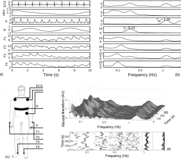
Several noninvasively measured signals of cardiovascular origin were recorded si-multaneously at different sites of the human body (Fig. 2(c)). The electrical activity of the heart (ECG), blood pressure, respiration and peripheral blood flow were mea-sured. The ECG was recorded by a standard instrument with electrodes on both shoulders and one below the heart. Piezoelectric sensors were used to detect the blood pressure and respiratory movements of the thorax. The peripheral blood flow was measured by the laser-Doppler technique3) on four different sites with similar density of vessels and network resistance.

Data were recorded for healthy young male subjects in repose. Each subject lay still on a bed, and was asked to relax: 15 minutes elapsed prior to the recording period of 20 minutes. The signals were digitized with 16 bit resolution: the ECG, blood pressure and respiration at 400 Hz sampling rate and blood flow at 40 Hz. The heart rate variability (HRV), consisting of instantaneous heart beat frequency determined within two consecutive R peaks, was derived from the ECG. A typical 10 s insert of all signals is shown in Fig. 2(a).

A time-averaged wavelet transform for each signal is presented in Fig. 2(b). Here, we cut off the low frequency band below 0.05 Hz and the high frequency band above 2.2 Hz. Within these boundaries three peaks can be found in all signals, except: in the respiratory signal, where the characteristic frequency of respiration dominates (fr ≈0.19 Hz), in the blood pressure signal where the heart beat frequency and its first harmonic dominate (fhb,2fhb;fhb ≈ 1.16 Hz), and in the HRV signal where, because of the way in which it is generated, the highest possible spectral frequency isfhb/2. The heart and the respiratory oscillations are both centrally generated and are then propagated within the network of vessels. The third frequency (≈0.1 Hz) originates locally — in the vessels’ walls. The continuous response of smooth muscle cells in the walls to changes in intravascular pressure is known as the myogenic response.20) There is no central source of oscillations of frequencyfm≈0.1 Hz, but

they originate from the cyclical contraction and relaxation of smooth muscle fibers which are spatially distributed throughout the entire vessels’ network, including the cardiac muscle.

−20 2

ECG

1 1.1 1.2

HRV

0 1

P

−1 0 1

R

8 12

F1

6 10

F2

4 10

F3

0 2 4 6 8 10

2 6

F4

Time (s)

0 5

0 5

0 5

0 10

0 10

0 10

0 5 10

0 5 10

1 0.3

0.1

Frequency (Hz) f

hb≈ 1.16

f r≈ 0.19

(a) (b)

Fig. 2. (a) A sequence of time series measured simultaneously: ECG — electrical activity of the heart, HRV — heart rate variability obtained as instantaneous frequency of the heart beat defined by anR-R interval, P — blood pressure and F1-F4 — peripheral blood flow. (b) Time averaged wavelet transforms calculated from time series recorded for 20 minutes. (c) Position of the sensors. (d) Wavelet transform of the blood flow signal (F₃) measured on the left leg and its time-frequency projection. The frequency bands for each of the three oscillatory components: cardiac (varying around 1.16 Hz), respiratory (varying around 0.2 Hz) and myogenic (varying around 0.1 Hz) are depicted. They are defined as a minimal window within which the maximal amplitude of each of the oscillatory component is to be found at any instant of time.

in the frequency interval of interest (whose lower limit corresponds to the one minute needed on average for the total amount of blood to circulate once through the sys-tem3),5): see above). It was shown that between 0.0095 Hz and 1.6 Hz the frequencies of the peaks in time-averaged wavelet transform derived from a number of subjects lie in distinct clusters. Each peak was shown to be located in the same frequency range in all measured subjects.5)

The heart-beat frequency is the highest frequency in the blood distribution sys-tem. Spectral peaks above 1.6 Hz are high harmonics of fhb. On the other side, a

repetition times longer than one minute.

In what follows we shall see whether some of the oscillations are spatially syn-chronized. For the sake of simplicity, relations among just three of them — the two centrally generated oscillations (heart and respiratory) and one peripherally gener-ated oscillation (the myogenic) — will be considered.

§4. Analysis of synchronization

There are two main methods to determine the instantaneous phase and frequency of an oscillatory process, based on (i) marker events, and (ii) analytic signal.

Marker events. We mark events that determine one cycle of oscillation. The phase and the frequency marked by two successive events are then linearly inter-polated to obtain their instant values. A 2π increase of phase is attributed to the interval between subsequent marker events. Hence, we can assign to the time ofk-th marker event,tk, the phase value φ(t) = 2πk, and

Φ(t) = 2π t−tk

tk+1−tk + 2πk, tk≤t < tk+1. (4.1)

Defined in this way the phase is a monotonically increasing piecewise-linear function of time defined on the real line.

Minimal or maximal values are usually taken as marker events. For instance, the peak value of the blood pressure signal, corresponding to a heart beat, is easily distinguishable and can be automatically detected. The same can be done for the ECG signal, where theR-peak is strongly pronounced and can also be automatically detected. The marker event approach can be applied easily in the case of signals where one oscillatory component dominates. However, not all processes in the blood distribution system can be measured selectively. Most of the quantities that can be measured, such as peripheral blood flow, contain multiple oscillatory processes and minima and maxima are no longer uniquely determined.

Analytic signal method. From the signal under observation, s(t), we construct an analytic signal, which is a complex function of time

ζ(t) =s(t) +i sH(t) =A(t)eiΦ(t). (4.2) The function sH(t) is the Hilbert transform ofs(t): A(t) and Φ(t) are the instan-taneous amplitude and the instaninstan-taneous phase. This method was originally intro-duced by Gabor18) and brought into the context of synchronization by Rosenblum, Pikovsky et al.10),13)-16) Although formallyA(t) andΦ(t) can be calculated for an arbitrary s(t), they have clear physical meaning if s(t) is a narrow-band signal.19) In this case the amplitudeA(t) coincides with the envelope ofs(t), and the instanta-neous frequency corresponds to the frequency of the maximum in the instantainstanta-neous spectra.

to calculate the instantaneous phase and frequency of: cardiac oscillations in the blood pressure and blood flow signals; respiratory oscillations in the blood pressure, blood flow, respiratory and HRV signals; and myogenic oscillations in the blood flow and HRV signals. The signals were band-pass filtered in the frequency domain, by assigning zero values to all amplitudes outside the interval from 0.913 Hz to 1.36 Hz for cardiac oscillations, from 0.137 Hz to 0.248 Hz for respiratory oscillations, and from 0.067 Hz to 0.137 Hz for myogenic oscillations. The phases were left unchanged. The limits for each of the oscillatory processes in time-averaged wavelet trans-forms of signals measured in a young healthy subject are marked in Fig. 2(b). The limits were determined by following the corresponding peak in the time-frequency plane of the wavelet transform of each signal. An example with the transform of one of the blood flow signals is presented in Fig. 2(d). In this way an optimal distinc-tion between two neighboring oscillatory processes, the myogenic and respiratory in particular, was achieved, keeping the band of each of the oscillatory processes narrow.

In Fig. 3 the instantaneous phase of cardiac oscillations obtained in two ways, using marker events and analytic signal method, is presented. In the first approach, the maximal values in the blood pressure signal are marked and taken as the instance when the phase is either 0 or 2π. In the second approach, the blood pressure signal is filtered to obtain the part that contains the cardiac frequency band only and than the instantaneous phase is calculated using the analytic signal method. Although the phases estimated in different ways slightly differ, their difference is constant in time. This difference illustrates the maximal systematic error that can occur. It results from both the difference in the methods applied, and the difference in the analysed signals in the time domain.

0 1 2 3 4 5

0 5

Time (s) (a)

0 1 2 3 4 5

0 π 2π

Time (s)

Φ

(b)

−π −π/2 0 π/2 π0 500

1000

Ψ_1,1

(d)

0 200 400 600 800 −π

0 π

Ψ1,1

(c)

0 1 2

0 5

f /f

× 104 (f)

0 200 400 600 800

0.9 1 1.1

Time (s)

fhb1

/fhb2

(e)

4.1. Spatial synchronization or self-synchronization

Here we analyse the state of synchronization between the same component ex-tracted from different signals, either representing different physiological quantities, such as ECG, HRV, blood flow or pressure, or/and measured at different sites of the cardiovascular system. Let us first introduce the measure that will be used to characterise the strength of synchronization. Methods based on quantifying the distribution of phases were proposed.10),17) Several indices were introduced that quantify the deviation of the actual distribution of the phase difference from a uni-form one. We shall use the index based on conditional probability: the intervals of two phasesΦ1(tk) and Φ2(tk), [0, n2π] and [0, m2π], are divided into N bins. Then we calculate

rl(tk) = 1

Ml

eiΦ2(tk)_{, 1≤l≤N (4.3)}

for all k such that Φ1(tk) belongs to bin l and Ml is the number of points in this

bin. If the phase difference is constant for all time, the two phases are completely dependent and |rl(tk)|= 1, whereas it is zero if there is no dependence at all. To

improve the statistics we average over all bins and obtain the synchronization index

λn,m = 1

N

N

l=1

|rl(tk)|. (4.4)

To analyse self-synchronization we chosen=m= 1. 4.1.1. Cardiac oscillations

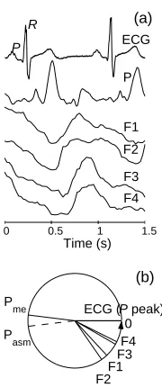
0 0.5 1 1.5

Time (s) (a)

(b)

0 ECG ( peak) P P

me

P asm

F2 F1

F4 F3 P

R

ECG

P

F1

F2

F3

F4

Fig. 4. Measured signals within one cardiac cycle (a) and the phase difference (b).

Measured signals during one cardiac cycle are presented in Fig. 4(a). The peaks P and R in the ECG correspond to the excitation and activation of atria and ventricles, respectively. We are in-terested in whether the electrical acti-vation of the heart is synchronized to the peak value that occurs in the pres-sure and flow signals with the cardiac frequency. For this reason we shall de-note the phase of a P-peak as a zero phase. The instantaneous phase and frequency were calculated either using marker events (in the ECG and blood pressure signal), or using analytic signal method after band pass filtering from 0.91 to 1.36 Hz.

difference was also obtained for all combinations with the value of the synchronization index lying between 0.96 and 0.99. The average phase differences are summarised in Fig. 4(b). The phase shift of the pressure wave is estimated in two ways: P_me — by marker events method applied on the measured signal directly; and P_asm — by the analytic signal method applied to the blood pressure signal after filtering. The pressure wave, recorded on the left second finger, is shifted by ∼π with respect to the initial phase of activation of the atria (the P-peak in the ECG). The interval between P and R peaks is known to be constant and is 150 ms for the measured subject. Therefore, theR-peak is also synchronized to the corresponding pressure or flow peak at all sites of the cardiovascular system. The phase difference π between the P-peak and the peak in the pressure corresponds to around 500 ms and about 350 ms between theR-peak and the peak in the pressure. We may take theR-peak as the moment when the pressure wave is generated, and it is then propagated to the point of measurement, around 70 cm away, at an average velocity 2 m/s.

The flow waves propagate at lower velocities, i.e. 22 cm/s in the aorta, the immediate artery starting from the heart, 8 cm/s in the vena cava that brings the blood to the heart, falling down to 0.3 mm/s in the smaller vessels. The closest point to the heart, where F₁ is measured, has the smallest phase difference, while the largest phase difference is observed with respect to the most distant measurement point from the heart — in the signal F₄ (measured over the ankle of the right leg, see Fig. 2(c)). However, the number of complete phase cycles over which a blood-flow wave oscillating at the cardiac frequency is propagated to distinct points of the peripheral vessels remains to be clarified.

4.1.2. Respiratory oscillations

0 5 10 15 20 25 Time (s)

R

HRV F1

F2

F3

F4

0 R F1 F3 F2 F4

HRV (a)

(b)

Fig. 5. Measured signals after filtering (a) and their average phase difference (b).

The respiratory synchronization was analysed using the analytic signal method. All signals were filtered so that only oscillations in the respiratory fre-quency range were left (Fig. 5(a)). The instantaneous frequency ratio, averaged over time, between any two of the mea-sured signals after band pass filtering from 0.137 to 0.248 Hz ranges from 0.96 (F₁and F₃) to 1.04 (HRV and F₁). This difference is within the limits of the cal-culation error. Hence, the instantaneous frequency of respiratory oscillations may be taken as the same, irrespective of the method or site of observation.

A preferred phase difference exists between any of the two signals, withλ1,1

ranging from 0.51 (R and F₁) to 0.86 (R and HRV). The average values of the

yet to be determined, since to our knowledge no data on the velocity of the respiratory wave propagation exist in the literature. In Fig. 6 typical time evolutions of the phase difference of two oscillatory components of respiratory origin, their frequency ratio and the index of synchronization are presented.

−π 0 π

Ψ 1,1

0 1 2

f r1

/f r2

0 200 400 600 800 1000 1200

0 0.5 1

Time (s)

λ 1,1

(a)

(b)

(c)

Fig. 6. Instantaneous phase difference (a), frequency ratio (b) and index of synchronization, com-puted in the running window [t−10, t+ 10], (c) between the respiration (R) and respiratory component into the blood flow measured on the skin over the right ankle joint (F3).

4.1.3. Myogenic oscillations

The myogenic activity cannot be measured selectively. As an oscillatory com-ponent with a basic frequency varying usually around 0.1 Hz it has been detected in the HRV, blood pressure and blood flow signal. Here we present analysis based on oscillatory component extracted from the HRV and four blood flow signals by band pass filtering from 0.0167 to 0.137 Hz (Fig. 7(a)).

0 10 20 30 40 50 Time (s)

0 HRV

F1 F2 F4 F3

HRV

F1

F2 F3

F4 (a)

(b)

Fig. 7. Measured signals after band pass fil-tering from 0.0167 to 0.137 Hz(a) and their average phase difference (b).

The average frequency ratio be-tween any pair of the analysed signals ranges from 0.92 Hz between the HRV and the second flow (F₂) to 1.23 Hz be-tween the flow on the left wrist (F₂) and the right ankle joint (F₃). This spa-tial variation of the basic frequency most probably reflects the local origin of the myogenic oscillations.

Also the synchronization index is lower for the myogenic oscillations, com-pared to indices for cardiac and respi-ratory oscillation. The obtained distri-bution of φ1,1 for all possible

combina-tions is nonuniform; however it largely fluctuates around a constant value. λ1,1

ranges from 0.22 for myogenic adjust-ment in the F₂ and F₄ signals to 0.47 for myogenic adjustment regarded from

shows average phase difference obtained for each of the analysed signals.

It is likely that the velocity of myogenic propagation is related to the time of myogenic oscillation (on average it takes 10 s for one cycle) and cannot be expected that one wave propagates within one cycle to any distinct point of the cardiovascular network. Therefore, the weaker spatial synchronization obtained for the myogenic component may well be on account of phase differences longer than 2π, as well as the local origin of the oscillations. A typical time-evolution of phase difference (a), frequency ratio (b) and synchronization index (c) for the myogenic component is presented in Fig. 8 illustrating the extent of instantaneous spatial adjustment of the myogenic activity.

−π 0 π

Ψ 1,1

0 2 4

f m1

/f m2

0 200 400 600 800 1000 1200

0 0.5 1

Time (s)

λ 1,1

(a)

(b)

(c)

Fig. 8. Instantaneous phase difference (a), frequency ratio (b) and synchronization index computed in the running window [t−20, t+ 20] (c). The myogenic components in the HRV and the blood flow (F₃), measured on the skin over the right ankle joint are used.

§5. Summary and outlook

We have used the concept of synchronization analysis developed for coupled nonlinear noisy oscillators to study spatial synchronization of oscillations in the cardiovascular system. The cardiac and respiratory systems generate pressure and flow oscillations which propagate throughout the entire system. Observed at different sites, in healthy subjects in repose, their oscillatory components appear to be strongly frequency and phase synchronized.

The myogenic oscillations are generated by the smooth muscle fibers in the vessel’s walls and are manifested via the elasticity of the vessels. They serve for local adjustment of the vessels’ radii and by this the system resistance. At different sites of the system they appear at the same or similar frequencies; however, at best, they are only weakly spatially phase synchronized.

Acknowledgements

We gratefully acknowledge P. V. E. McClintock and M. Braˇciˇc-Lotriˇc for valuable comments on the manuscript. The study was supported by the Slovenian Ministry of Science and Technology.

References

1) R. M. Berne and M. N. Levy (ed.),Physiology(Mosby, St. Louis, Missouri, 1998). 2) H. D. Kvernmo, A. Stefanovska, K. A. Kirkebøen and K. Kvernebo, Microvasc. Res.57

(1999), 298.

3) A. Stefanovska and M. Braˇciˇc, Contemp. Phys.40(1999), 31.

4) A. Syefanovska, M. Braˇciˇc and H. D. Kvernmo, IEEE Trans. Bimed. Eng.46(1999), 1230. 5) M. Braˇciˇc, P. V. E. McClintock and A. Stefanovska, in preparation. (2000).

In D. S. Broomhead, E. A. Luchinskaya, P. V. E. McClintock and T. Mullin (ed.), Stochas-tic and ChaoStochas-tic Dynamics in the Lakes(American Institute of Physics, Melville, New York, 2000), p. 146.

6) C. Sch¨afer, M. G. Rosenblum, J. Kurths and H.-H. Abel, Nature392(1998), 239. 7) C. Sch¨afer, M. G. Rosenblum H.-H. Abel and J. Kurths, Phys. Rev.E60(1999), 857. 8) M. Braˇciˇc and A. Stefanovska, Nonlinear Phenomena in Complex Systems (2000), in press. 9) C. H. Hugenii (Huygens),Horologium Oscillatorium(Apud F. Muguet, Parisiis, France,

1673).

10) M. G. Rosenblum, A. S. Pikovsky, C. Sch¨afer, P. Tass and J. Kurths,Handbook of Biological Physics, ed. F. Moss (Elsevier, 2000).

11) A. Stefanovska, S. Strle, M. Braˇciˇc and H. Haken, Nonlinear Phenomena in Complex Systems2(1999), 72.

12) V. I. Arnold,Mathematical Methods of Classical Mechanics(Springer-Verlag, New York, 1978).

13) M. G. Rosemblum, A. S. Pikovsky and J. Kurths, Phys. Rev. Lett.76(1996), 1804. 14) A. S. Pikovsky, M. G. Rosemblum and J. Kurths, Europhys. Lett.34(1996), 165. 15) M. G. Rosemblum, A. S. Pikovsky and J. Kurths, Phys. Rev. Lett.78(1997), 4193. 16) A. S. Pikovsky, M. G. Rosemblum, G. V. Osipov and J. Kurths, PhysicaD104(1997),

219.

17) P. Tass, M. G. Rosemblum, J. Weule, J. Kurths, A. S. Pikovsky, J. Volkmann, A. Schnitzler and H.-J. Freund, Phys. Rev. Lett.81(1998), 3291.